Sometimes it is useful to extract table names from an SQL statement,
for example if you are trying to figure out dependencies for your Hive
or BigQuery (or whatever) tables.
It is actually a lot simpler than it seems and you don’t need to write
your own SQL parser or find one out there. In SQL table names always
follow the FROM and JOIN keywords. So all you have to do is split the
statemement into tokens, and scan the list for any mention of FROM or
JOIN and grab the next token.
Here is a very simplistic Python function that does this using regular
expressions:
123456789101112131415161718192021222324252627
deftables_in_query(sql_str):# remove the /* */ commentsq=re.sub(r"/\*[^*]*\*+(?:[^*/][^*]*\*+)*/","",sql_str)# remove whole line -- and # commentslines=[lineforlineinq.splitlines()ifnotre.match("^\s*(--|#)",line)]# remove trailing -- and # commentsq=" ".join([re.split("--|#",line)[0]forlineinlines])# split on blanks, parens and semicolonstokens=re.split(r"[\s)(;]+",q)# scan the tokens. if we see a FROM or JOIN, we set the get_next# flag, and grab the next one (unless it's SELECT).result=set()get_next=Falsefortokintokens:ifget_next:iftok.lower()notin["","select"]:result.add(tok)get_next=Falseget_next=tok.lower()in["from","join"]returnresult
This is obviously not perfect, for example in BigQuery there is a
possibility that what follows SELECT is a UDF name, but I’ll leave
working around that as an exercise for the reader.
So I finally got around to some load testing of Tgres. Load testing is
mysterious, it never goes the way you think it would, and what you
learn is completely unexpcted.
Given that I presently don’t have any spare big iron at my disposal
and my “servers” are my macbook and an old thinkpad, all I really was
after is making sure that Tgres is “good enough” whatever that
means. And I think it is.
I was hoping to gather some concrete numbers and may be even make a
chart or two, but in the end it all turned out to be so tedious and
time consuming, running the tests with various setting for hours on,
that I just gave up for now - after all, “premature optimization is
the root of all evil”.
I also wanted to see how it stacks up against Graphite
carbon-cache.py. As in, is it on par, or much better or much worse. My
expectation was that Graphite could outperform it, because what it
does is so much simpler (and I was right). First thing I tried to do
is overwhelm Graphite. I never succeeded in that - I probably could
have tried harder, but I quickly learned that I don’t know what
symptoms I’m looking for. I wronte a Go program that blasted UDP data
points at 10K/sec across 10K different series, and taking it to over
20K/sec saturated my network before Graphite showed any signs of
deterioration. There was also no reliable way for me to audit the data
points - may be some of them got lost, but at 600K+ per minute, I
don’t know of any practical way of doing it. Not without a lot of
work, at least.
With Tgres things were much easier. The weakest link is, not
surpisingly, PostgreSQL. What I learned was that there are two kinds of
deterioration when it comes to PostgreSQL though. The first one is
outright, and that one manifests in database requests getting
progressively slower until Tgres gets stuck with all its channels
full.
You can make PostgreSQL very significantly faster with a few simple
tricks. For example the following settings can make it much faster:
12
synchronous_commit = off
commit_delay = 100000
This post isn’t about PostgreSQL, and so I’m not going to get into the
details of what this does, there is plenty of documentation and blog
posts on the subject. If you plan on hosting a busy Tgres set up, you
should probably have the above settings.
The second way PostgreSQL deteriorates is not immediately apparent - it
is the infamous table bloat. Getting autovacuum to keep up with the ts
table (which stores all the time series) is tricky, and once you’ve
ran out of options to tweak, this is probably it - the maximum load
the database can handle, even if it may seem relatively calm.
Autovacuum has a lot of knobs, but ultimately they all exist to take
advantage of the variability of load in a database, i.e. you can let
it get behind during the day and catch up at night when the database
is not as busy. It doesn’t really work with time series, which are not
variable by nature - if you’re receiving 5 thousand data points per
second at noon, you can expect the same rate at 4am. I think the
setting that worked best for me were:
To the best of my undestanding the above setting disables cost-based
autovacuum (meaning it doesn’t pause periodically to yield resources
to the normal db tasks), makes autovacuum kick in after 2K updates
(which happens in no time), and sleeps 1s in between runs, which means
it’s running pretty much continuosly.
I was able to sustain a load of ~6K datapoints per second across 6K
series - anything higher caused my “database server” (which is a 2010
i7 Thinkpad) autovacuum to get behind.
I also did some testing of how TOAST affects performance. There is no
setting for turning TOAST on or off, but it can easily be done in
Tgres by changing the number of data points per row. The default is
768 which is about 75% of a page. If you for example double it, then
each row becomes larger than a page and TOAST kicks in. TOAST is
compressed, which is an advantage, but it is a separate table, which
is a disadvantage. In the end it seemed like the database detirorated
quicker with TOAST, but it was rather inconclusive.
In the end the key factor, or the weakest link, was the rate of
queries per second. I now added a special rate limiting setting
feature to Tgres (max-flushes-per-second) which trumps all other
settings and will keep your database happy at the expense of Tgres
possibly caching a little more points in memory than expected.
I will probably get back to some more load testing in a while, but for
now this is it.
What is the difference between a Go receiver (as in “method receiver”)
and a function argument? Consider these two bits of code:
123
func(d*duck)quack(){// receiver// do something}
versus
123
funcquack(d*duck){// funciton argument// do something}
The “do something” part above would work exactly the same regardless of
how you declare the function. Which begs the question, which should
you use?
In the object-oriented world we were used to objects doing things, and
in that context d.quack() may seem more intuitive or familiar than
quack(d) because it “reads better”. After all, one could argue that
the former is a duck quacking, but the latter reads like you’re
quacking a duck, and what does that even mean? I have learned that you
should not think this way in the Go universe, and here is why.
First, what is the essential difference? It is that at the time of the
call, the receiver is an interface and the function to be called is
determined dynamically. If you are not using interfaces, then this
doesn’t matter whatsoever and the only benefit you are getting from
using a method is syntactic sweetness.
But what if you need to write a test where you want to stub out
quack(). If your code looks like this, then it is not possible,
because methods are attached to their types inflexibly, you cannot
change them, and there is no such thing as a “method variable”:
12345678910
typeduckstruct{}func(d*duck)quack(){// do something}// the function we are testing:functestme(d*duck){d.quack()// cannot be stubbed}
However, if you used a function argument, it would be easy:
12345678910
typeduckstruct{}varquack=func(d*duck){// do something}// the function we are testing:funcfoo(d*duck){quack(d)}
Now you can assign another function to quack at test time, e.g. quack = func(d *duck) { // do something else } and all is
well.
Alternatively, you can use an interface:
1234567891011121314
typequackerinterface{quack()}typeduckstruct{}varfunc(d*duck)quack(){// satisfies quacker// do something}// the function we are testing:funcfoo(dquacker){d.quack()}
Here, if we need to test foo() we can provide a different
quacker.
Bottom line is that it only makes sense to use a receiver if this
function is part of an interface implementation, OR if you never ever
need to augment (stub) that function for testing or some other
reason. As a practical matter, it seems like (contrary to how it’s
done in the OO world) it is better to always start out with quack(d)
rather than d.quack().
This silly SVG animation (animation not my strong suit) demonstrates
what happens when multiple Tgres data points arrive within the same
step (i.e. smallest time interval for this series, also known as PDP,
primary data point).
Explanation
Let’s say we have a series with a step of 100 seconds. We receive the
following data points, all within the 100 second interval of a
single step:
Time
Value
Recorded
25s
2.0
0.5
75s
3.0
2.0
100s
1.0
2.25
Final:
2.25
Tgres will store 2.25 as the final value for this step. So how
does 1, 2 and 3 add up to 2.25?
One way to think about it is that the incomplete step is an empty
swimming pool as wide as 1 step, into which we dump blocks of
water. The first data point dumps a 2.0 × 0.25 block of water, which
fills the pool to 0.5. The second data point dumps a 3.0 × 0.50 block,
which raises the water another 1.5 to 2.0. The last data point dumps a
1.0 × 0.25 block which raises it to the final value of 2.25. Compare
this with Graphite which would simply discard the first two data
points and we are left with 1.0 as the final value.
Why is it done this way? Because this is how rates add up. If this was
speed of a car in meters per second (more like a bycicle, I guess),
its weighted average speed for the duration of this step of 2.25
meters per second would mean that in the 100s it would have traveled
exactly 225 meters.
NaNs or “Unknowns”
What if instead of the first data point, the first 25s were “unknown”
(recorded as NaN)? This would happen, for example, if the series
heartbeat (maximum duration without any data) was exceeded. Even
though the data point has a value of 2.0, it gets recorded as NaN.
Time
Value
Recorded
25s
2.0
NaN
75s
3.0
2.0
100s
1.0
2.33
Final:
2.33
But wait a second… 0.50 × 3 + 0.25 × 1 = 1.75 ? Where did
the value of 2.33 come from?
The reason for this is that NaN ought not be influencing the
value. The above calculation would only be correct if we assumed that NaN is
synonymous with zero, but that would be a false assumption, as NaN
means “we do not know”.
Therefore, we must only consider the known part of the data point,
which is 75s. We can think of it that the data point (the “swimming
pool”) just got smaller. Thus the correct calculation for the 3.0
point would be 3.0 × 50 ÷ 75 = 2.0 and for the 1.0 point
2.0 + 1.0 × 25 ÷ 75 = 2.33.
Here it is in SVG:
Also note how the value of the data point which was recorded as NaN
(2.0 in our example) is essentially irrelevant. This is because any
calculation with a NaN always results in a NaN. The only thing we know
about this data point is that it was not NaN and that it marked the
end of period recorded as NaN. The next data point after this (3.0 in
our example) is not affected by the NaN, however, this is because it
in effect starts its own data point afresh, not considering anything
in the past.
Tgres is a metrics collection and storage server, aka a time series
database. I’m not very comfortable with referring to it as a
database, because at least in case of Tgres, the database is
actually PostgreSQL. But also “database” to me is in the same category
as “operating system” or “compiler”, a thing so advanced that only few
can claim to be it without appearing pretentious. But for the sake of
tautology avoidance, I might occasionally refer to Tgres as a TS
database.
Ulike Graphite or
RRDTool, Tgres produces no charts,
it assumes you’re using something like
Grafana. Currently Tgres supports most of the
Graphite functionality (including vast majority of the functions) as
well as Statsd functionality. Tgres supports clustering, albeit
whereby all nodes must share the PostgreSQL instance. Tgres can be
used as a standalone server or as a Go package compiled into your app.
Current status
It’s been over a year since I began hacking on it in this incarnation,
though the idea and a couple of scrapped implementations thereof go
back more than two years. Tgres is still not quite production quality,
though it’s probably stable enough for someone who knows their way
around Go to give it a whirl. At this point I have proven the concept,
and believe the architecture is sound, but the magnitude of the
project turned out to be much grater than I originally pictured, and
so it still needs lots and lots of proofreading, t’s crossed and i’s
dotted.
Raisons d’etre
With Go, new things are possible
The idea of a TS database came about when I first decided to dive into
Golang. Go can do great stuff, but I didn’t see
how it applied to anything I was working on at
the time. I needed a project that was a better match for the domain of
applications that Go made possible, something where performance and scale
matter, something with concurrent moving pieces, something
challenging. A “time series database” seemed like it had potential. It
has all kinds of curious requirements that could be great fun to
implement in Go.
Present state of “time series databases” is dismal
I was (and still am) frustrated with the state of TS in our
industry. Since the appearance of
MRTG back in 1995 when
the network admins of the then burgeoning Internet realized that TS is
essential to device monitoring, not much has happened.
RRDTool was definitely a major step
forward from MRTG which was merely a Perl script. RRDTool to this day
is the best implementation of a round-robin database for time series
data (in C to boot). Similarly to MRTG, RRDTool was designed as a command-line tool,
the server component was left as an exercise for the user. And even
though linking RRDTool into your app was not too difficult (I
did it
in 2004), somehow an “RRD server” never appeared.
Then there was Graphite. (I think Graphite
is a reflection of the Python-can-do-anything era.) Graphite borrowed
a lot of ideas from RRDTool, though its re-implementation of
round-robin on-disk files in pure Python while claiming superiority is not that much
better, if at all, IMHO when compared to RRDTool in both accuracy and
performance. In general though, I think storing data directly in files
is the wrong approach to begin with.
Graphite’s appeal is that it’s an easy-to-start server that does
everything, and it became especially popular alongside
Statsd a tool with umpteen
different implementation designed to sit in front of
Graphite. Eventually people stopped using Graphite to make charts
favoring instead the most excellent Grafana,
while Graphite (or its nephew Graphite-API)
became a UI-less server-only component to store and retrieve data.
Graphite and RRDTool didn’t scale very well, so for “Big Time Series”
(as in very large networks, or specialized fields like finance,
weather, etc.) people used solutions backed by
Cassandra, HBase,
or Solr such as
OpenTSDB.
There are also new kids on the block such as
InfluxDB or
Prometheus, which are a little too flashy
and commercial by my taste, each trying to solve problems that I don’t
think I have.
Bottom line is that some 20 years after MRTG, time series remains
mostly a system monitoring aid and has never crossed over to the
mainstream application development.
Data isolation
Virtually all of the aforementioned tools contribute to a problem I
dub data isolation. Data isolation is when a part of our data is
stored using a separate tool in a different format and is therefore
not as easily accessible. For example if our metrics are in Graphite,
we probably don’t even know how to get them out of it, nor does it
occur to us that it might be useful. All we’ve been able to do is get
a Grafana chart and are quite satisfied with it. We do not question
why it isn’t a first-class citizen right in the database as a table,
where we could use it in SQL joins, for example. Or export it to our
big data rig and query it with Hive or Spark, etc.
Why is getting a quick chart of customer sign-ups per second next to
all my customer data such a big deal these days? Why can’t it be as
simple as a model in my Rails or Django app?
PostgreSQL - Avoid the storage mire
I believe that there is nothing about time series that makes it unfit
for a relational database. Many projects out there are spinning
their wheels solving the wrong problem, that of data storage. Storage
is one of the hardest problems in computers, time series databases
should focus on time series and delegate the storage to tried-and-true
tools which are good at it.
Time series data does carry certain special requirements, and I’ve
researched extensively all different ways TS can be stored in a
relational database. It does require taking advantage of some newer
features that in the open source database world seem most available in
PostgreSQL. I am guessing that with time these capabilities will
become more available in other databases, and some of them already
are, but for the time being I’ve decided that Tgres is
PostgreSQL-only.
A bit of detail
Emulating Graphite as a starting point
I would like Tgres to be useful. The simplest way I could think of
achieving usefulness is by emulating an existing tool so that it can
become a drop-in replacement. This makes adoption easy and it also
proves that the underlying architecture is capable. It also lets us
compare performance.
It doesn’t mean that I am a fan of how Graphite does things, but I
think that if Tgres is architected in such a way that there is a lower
level which does the heavy lifting and then a layer on top of it that
makes it behave like Graphite, that’s a great start, and it leaves
options open for potential improvement and a different/better
interface.
General terminology
I always liked how RRDTool documentation broke down the problem of
time series into concise and clear terms. Tgres tries to leverage the
RRDTool terminology. Tgres also adopts the same techniques to the
extent that is possible given a considerably different
architecuture. Unlike RRDTool, Tgres uses a millisecond as the
smallest unit of time measure.
Data Point (DP)
A data point is a value (a floating point number) a time stamp
and a string name identifying the series. (For a while I
contemplated allowing a data point to have multiple values, but it
made things too complicated, so I reverted to a single value per data
point).
Round-Robin Archive (RRA)
Tgres stores data points in round-robin archives. While
“round-robin” is an implementation detail, it is part of the name
because the only way it can be round-robin is the number of data
points in the archive is constant. The time-span of the RRA is determined
by the step (resolution) and the size of the archive (in steps). Thus RRA’s are
defined by step and size, e.g. 10s for 24 hours (a data point every
10s for 24 hours, or 8,640 points).
A series is usually is stored in multiple RRA’s. The RRA’s typically
have varying resolutions, e.g. we want a 10s step for the past 24h,
but also a 1h step for a week and a 6h step for 3 years. In this
example we have 3 RRA’s. Tgres takes care of maintaining the RRA’s and
selecting the right resultion for a given query so that there is no
need to deal with individual RRA’s directly.
Data Source (DS)
A group of RRA’s under the same identifier (aka series name) is
referred to as a data source (DS). I suppose “DS” can be used
interchangeably with “series”. Depending on how Tgres is configured,
DS’s are either predefined or are created on the fly based on DS name
matching rules.
Note that Tgres does not store the original data points, but only the
weighted averages of the received data points in each RRA. This is how
RRDTool does it. Graphite doesn’t bother averaging the points but
simply discards previous data points within the same step. At first it
may seem not ideal that the original data is discarded, but experience
shows that just about any time series operation results in a
conversion to a fixed interval form as the first step, so it might as
well just be done upfront.
Heartbeat (HB)
Every DS has a heartbeat, a time duration which defines the longest
possible period of inactivity before the DS becomes considered
dysfunctional. If the heartbeat is exceeded, the data since the last
update will be recorded as NaNs.
Xfiles factor (XFF)
When data is consolidated from smaller to larger step RRAs, the XFF
determines how much of the data is allowed to be NaN before the
consolidated value becomes NaN. For example if we are consolidating
per-minute values into a per-hour value, if one of the minutes happens
to be NaN, strictly speaking the whole hour ought ot be NaN, but that
wouldn’t be very useful. Default XFF is .5, i.e. more than half of the
per-minute values should be NaN before the per-hour value is
considered NaN.
Postgres storage format
A time series is a series of floats. Note that when it’s stored in
RRA’s, there is no need for timestamps - each position in an RRA has
its timestamp defined by the current state of the RRA. If we know the
timestamp of the tip, we know the timestamp of every element going
back to the beginning of the RRA.
To store data points Tgres takes advantage of PostgreSQL arrays. A
single row stores many data points. Tgres further splits series into
multiple rows to optimize the IO.
To make the data easy to use, Tgres also creates a view which makes
the data points structured as a regular table with a row per data
point.
There are only 3 tables and 1 view required for Tgres operation. You
can use the same database you use for any other web app you have. This
means you can access the time series by simply just adding a model
pointing at the Tgres time series view to your Rails/Django/whatever
to get access to the data.
Tgres components
Tgres is organized as a set of Go packages.
tgres/daemon
The daemon is the
main process that runs everything. It includes the config parser, and
the listeners that receive and parse incoming data points using both
UDP and TCP Graphite formats, as well as Python Pickle format (though
I’m not sure who out there really uses it). It’s not too hard to add
more formats, for example I think it’d be neat if Tgres could receive
data points via an HTTP pixel that could be embedded in web pages.
The daemon also takes care of graceful restarts, logging and other
typical long-running service stuff.
trges/receiver
The receiver
(formerly known as transceiver) is the data point router and cache. It
maintains a set of workers responsible for writing the data points to
their respective RRA’s, as well as caching and periodic flushing of
the cache. Flushing is done once a certian number of points has
accumulated or a period of time has passed, but not more often than
the minimal flush frequency (all configurable).
tgres/rrd
The responsibility of rrd is to add data
points to RRA’s. This is not as simple as it sounds, a good
description of the concepts behind it is available here.
tgres/http
http is the place
for all things related to HTTP, which currently is just the Graphite
API. The API requests are passed down to the DSL level for processing.
tgres/dsl
dsl is an
implementation of the Graphite
functions. There
are a few differences because I used the Go parser which is nearly
syntactically identical. (For example a series name cannot begin with
a digit because that is not a proper Go identifier).
Graphite has a lot number of functions available in its DSL, and I
spent a lot of time during our beach vacation last summer trying to
implement them all, but I think a few are still left undone. Some were
harder than others, and some led me on side adventures such as
figuring out the Holt-Winters triple exponential smoothing and how to
do it correctly. (ZZZ - link)
tgres/serde
The interface to the database is reduced to a fairly compact
SerDe
(Serialize-Deserializer) interface. While the SerDe itself is utterly
simplistic (e.g. “get me this series”), the SQL behind it anything
but, still, it should be possible to throw together an alternative
SerDe for a different relational database (or not a database at all?).
tgres/statsd
Statsd is currently
in a separate Go package, but I might integrate with the RRD because
it is not very clear that it needs to be a separate thing. Somehow it
so happened that Graphite and Statd are two separate projects, but the
reasons for this are probably more cultural than by design.
tgres/cluster
Cluster supports
very basic clustering. At this point it’s “good enough” given that
it’s OK to occasionally lose data points during cluster transitions
and all that we want to make sure of is that nodes can come and go
without disruptions.
The principle behind cluster is that each node is responsible for one
or more series and other nodes will forward data points to the
responsible node. There is nearly zero configuration, and any node can
act as the point of contact, i.e. there is no leader.
The way clustering is done is in flux at the moment, we might change
it to something more robust in the near future, but for the time being
it addresses the horizontal scaling problem.
There’s still lots to do…
There’s still a lot of work to be done on Tgres. For one thing, I
don’t have any tests. This is mainly because I don’t believe in
testing that which hasn’t “gelled”, and I wouldn’t be surprised if the
above organization of packages and how they interface changes as I
understand the problem better. We also need documentation. And some
real-life use/testing/feedback would be great as well.
I’ve put together a basic example of a “Hello World” Go program which
runs in Amazon AWS Elastic Compute Service (ECS), which allows running
applications in Docker containers and has the ability to scale on
demand.
I initially wanted to write about the components of this system and
the tools you use to deploy your application, but soon realized that
this would make for an extremely long post, as the number of
components required for a simple “Hello World” is mind
boggling. However problematic it may seem, it’s par for the course,
this is what takes to run an application in our cloudy times.
I used Terraform to build
all the AWS infrastructure. Initially I was skeptical on how well it
could accomplish such a tedious task, but I have say my confidence in
Terraform grew the more I used it.
The main top level tool for everything is the good old
make, a tool that
stood the test of time.
Here is the code of the example, read the README, I hope you find it
useful:
If you haven’t read Part I and
Part II
you probably should, or the following will be hard to make sense of.
In Part I we’ve learned how to forceast one point, in Part II we’ve
learned how to forecast two points. In this part we’ll learn how to
forecast many points.
More Terminology
Season
If a series appears to be repetitive at regular intervals, such an
interval is referred to as a season, and the series is said to be
seasonal. Seasonality
is required for the Holt-Winters method to work, non-seasonal series
(e.g. stock prices) cannot be forecasted using this method (would be
nice though if they could be).
Season Length
Season length is the number of data points after which a new season
begins. We will use $L$ to denote season length.
Seasonal Component
The seasonal component is an additional deviation from level + trend
that repeats itself at the same offset into the season. There is a
seasonal component for every point in a season, i.e. if your season
length is 12, there are 12 seasonal components. We will use $s$ to
denote the seasonal component.
The idea behind triple exponential smoothing is to apply exponential
smoothing to the seasonal components in addition to level and
trend. The smoothing is applied across seasons, e.g. the seasonal
component of the 3rd point into the season would be exponentially
smoothed with the the one from the 3rd point of last season, 3rd point
two seasons ago, etc. In math notation we now have four equations (see footnote):
What’s new:
We now have a third greek letter, $\gamma$ (gamma) which is the smoothing
factor for the seasonal component.
The expected value index is $x+m$ where $m$ can be any integer meaning
we can forecast any number of points into the future (woo-hoo!)
The forecast equation now consists of level, trend and the seasonal
component.
The index of the seasonal component of the forecast
$s_{x-L+1+(m-1)modL}$ may appear a little mind boggling, but it’s
just the offset into the list of seasonal components from the last set
from observed data. (I.e. if we are forecasting the 3rd point into the
season 45 seasons into the future, we cannot use seasonal components
from the 44th season in the future since that season is also
forecasted, we must use the last set of seasonal components from
observed points, or from “the past” if you will.) It looks much
simpler in Python as you’ll see shortly.
Initial Values
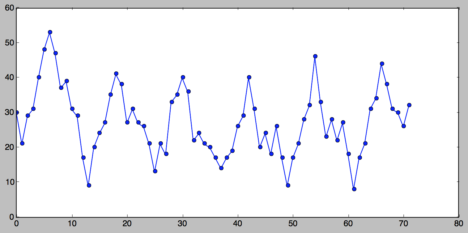
Before we can discuss initial values, let me introduce to you a new
tiny series (okay, not as tiny):
You can see that this series is seasonal, there are clearly visible 6
seasons. Although perhaps not easily apparent from the picture, the
season length for this series is 12, i.e. it “repeats” every 12
points. In order to apply triple exponential smoothing we need to know
what the season length is. (There do exist methods for detecting
seasonality in series, but this is way beyond the scope of this text).
Initial Trend
For double exponential smoothing we simply used the first two points
for the initial trend. With seasonal data we can do better than that,
since we can observe many seasons and can extrapolate a better
starting trend. The most common practice is to compute the average of
trend averages across seasons.
Good news - this looks simpler in Python than in math notation:
The situation is even more complicated when it comes to initial values
for the seasonal components. Briefly, we need to compute the average
level for every observed season we have, divide every observed value
by the average for the season it’s in and finally average each of
these numbers across our observed seasons. If you want more detail, here is
one thorough description of this process.
I will forgo the math notation for initial seasonal components, but
here it is in Python. The result is a season-length array of seasonal components.
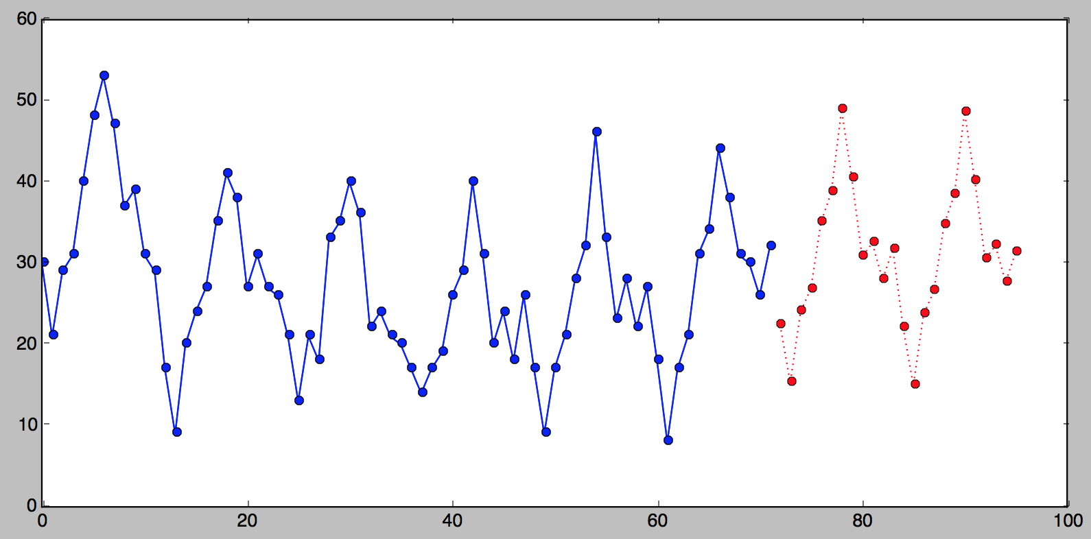
And finally, here is the additive Holt-Winters method in Python. The
arguments to the function are the series of observed values, the
season length, alpha, beta, gamma and the number of points we want
forecasted.:
1234567891011121314151617181920212223
deftriple_exponential_smoothing(series,slen,alpha,beta,gamma,n_preds):result=[]seasonals=initial_seasonal_components(series,slen)foriinrange(len(series)+n_preds):ifi==0:# initial valuessmooth=series[0]trend=initial_trend(series,slen)result.append(series[0])continueifi>=len(series):# we are forecastingm=i-len(series)+1result.append((smooth+m*trend)+seasonals[i%slen])else:val=series[i]last_smooth,smooth=smooth,alpha*(val-seasonals[i%slen])+(1-alpha)*(smooth+trend)trend=beta*(smooth-last_smooth)+(1-beta)*trendseasonals[i%slen]=gamma*(val-smooth)+(1-gamma)*seasonals[i%slen]result.append(smooth+trend+seasonals[i%slen])returnresult# # forecast 24 points (i.e. two seasons)# >>> triple_exponential_smoothing(series, 12, 0.716, 0.029, 0.993, 24)# [30, 20.34449316666667, 28.410051892109554, 30.438122252647577, 39.466817731253066, ...
And here is what this looks like if we were to plot the original
series, followed by the last 24 points from the result of the
triple_exponential_smoothing() call:
A Note on α, β and γ
You may be wondering how I came up with 0.716, 0.029 and 0.993 for
$\alpha$, $\beta$ and $\gamma$, respectively. To make long story short, it
was done by way of trial and error: simply running the algorithm over and
over again and selecting the values that give you the smallest
SSE. As I
mentioned before, this process is known as fitting.
To compute the smothing factors to three decimal points
we may have to run through 1,000,000,000 iterations, but luckily
there are more efficient methods at zooming in on best
values. Unfortunately this would take a whole other very long post to
describe this process. One good algorithm for this is
Nelder-Mead,
which is what tgres uses.
Conclusion
Well - here you have it, Holt-Winters method explained the way I wish
it would have been explained to me when I needed it. If you think I
missed something, found an error or a suggestion, please do not
hesitate to comment!
Footnote
The triple exponential smoothing additive method formula is as it is
described in “Forecasting Method and Applications, Third Edition” by
Makridakis, Wheelwright and Hyndman (1998). Wikipedia has a different
formula for the seasonal component (I don’t know which is better):
If you haven’t read Part I
you probably should, or the following will be hard to make sense of.
All the forecasting methods we covered so far, including single
exponential smoothing, were only good at predicting a single
point. We can do better than that, but first we need to be introduced to
a couple of new terms.
More terminology
Level
Expected value has another name, which, again varies depending on who wrote the
text book: baseline, intercept (as in
Y-intercept) or
level. We will stick with “level” here.
So level is that one predicted point that we learned how to calculate
in Part I. But because now it’s going to be only part of calculation
of the forcast, we can no longer refer to it as $\hat{y}$ and will instead
use $\ell$.
Trend or Slope
You should be familiar with
slope from your high school algebra
class. What you might be a little rusty on is how to calculate it,
which is important, because a series slope has an interesting
characteristic. Slope is:
where $\Delta{y}$ is the difference in the $y$ coordinates and
$\Delta{x}$ is the difference in the $x$ coordinates, respectively,
between two points. While in real algebraic problems $\Delta{x}$ could
be anything, in a series, from one point to the next, it is always
1. Which means that for a series, slope between two adjacent points
is simply $\dfrac{\Delta{y}} {1}$ or $\Delta{y}$, or:
Where $b$ is trend. To the best of my understanding terms “trend”
and “slope” are interchangeable. In forecasting parlance “trend” is
more common, and in math notation forecasters refer to it as $b$
rather than $m$.
Additive vs Multiplicative
Another thing to know about trend is that instead of subtracting
$y_{x-1}$ from $y_x$, we could divide one by the other thereby
getting a ratio. The difference between these two approaches is
similar to how we can say that something costs $20 more or 5%
more. The variant of the method based on subtraction is known as
additive, while the one based on division is known as
multiplicative.
Practice shows that a ratio (i.e. multiplicative) is a more stable
predictor. The additive method, however is simpler to understand, and
going from additive to multiplicative is trivial once you understand
this whole thing. For this reason we will stick with the additive
method here, leaving the multiplicative method an exercise for the
reader.
Double Exponential Smoothing
So now we have two components to a series: level and trend. In Part I
we learned several methods to forecast the level, and it should follow
that every one of these methods can be applied to the trend
just as well. E.g. the naive method would assume that trend between
last two points is going to stay the same, or we could average all
slopes between all points to get an average trend, use a moving trend
average or apply exponential smoothing.
Double exponential smoothing then is nothing more than exponential
smoothing applied to both level and trend. To express this in
mathematical notation we now need three equations: one for level, one
for the trend and one to combine the level and trend to get the
expected $\hat{y}$.
The first equation is from Part I, only now we’re using $\ell$ instead
of $\hat{y}$ and on the right side the expected value becomes the sum
of level end trend.
The second equation introduces $\beta$, the trend factor (or
coefficient). As with $\alpha$, some values of ${\beta}$ work better
than others depending on the series.
Similarly to single exponential smoothing, where we used the first
observed value as the first expected, we can use the first observed
trend as the first expected. Of course we need at least two points to
compute the initial trend.
Because we have a level and a trend, this method can forecast not one,
but two data points. In Python:
1234567891011121314151617
# given a series and alpha, return series of smoothed pointsdefdouble_exponential_smoothing(series,alpha,beta):result=[series[0]]forninrange(1,len(series)+1):ifn==1:level,trend=series[0],series[1]-series[0]ifn>=len(series):# we are forecastingvalue=result[-1]else:value=series[n]last_level,level=level,alpha*value+(1-alpha)*(level+trend)trend=beta*(level-last_level)+(1-beta)*trendresult.append(level+trend)returnresult# >>> double_exponential_smoothing(series, alpha=0.9, beta=0.9)# [3, 17.0, 15.45, 14.210500000000001, 11.396044999999999, 8.183803049999998, 12.753698384500002, 13.889016464000003]
And here is a picture of double exponential smoothing in action (the
green dotted line).
Quick Review
We’ve learned that a data point in a series can be represented as a
level and a trend, and we have learned how to appliy exponential
smoothing to each of them to be able to forecast not one, but two
points.
In Part III
we’ll finally talk about triple exponential smoothing.
This three part write up [Part IIPart III]
is my attempt at a down-to-earth explanation (and Python code) of the
Holt-Winters method for those of us who while hypothetically might be
quite good at math, still try to avoid it at every opportunity. I had
to dive into this subject while tinkering on
tgres (which features a Golang implementation). And
having found it somewhat complex (and yet so brilliantly
simple), figured that it’d be good to share this knowledge, and
in the process, to hopefully solidify it in my head as well.
Triple Exponential Smoothing,
also known as the Holt-Winters method, is one of the many methods or
algorithms that can be used to forecast data points in a series,
provided that the series is “seasonal”, i.e. repetitive over some
period.
A little history
Еxponential smoothing in some form or another dates back to the work
of Siméon Poisson (1781-1840),
while its application in forecasting appears to have been pioneered over a century later in 1956 by
Robert Brown (1923–2013)
in his publication
Exponential Smoothing for Predicting Demand,
(Cambridge, Massachusetts). [Based on the URL it seems Brown was working on forecasting tobacco demand?]
In 1957 an MIT and University of Chicago
graduate, professor Charles C Holt
(1921-2010) was working at CMU (then known as CIT) on forecasting trends in production,
inventories and labor force.
It appears that Holt and Brown worked independently and knew not of each-other’s work.
Holt published a paper “Forecasting trends
and seasonals by exponentially weighted moving averages” (Office of Naval Research Research
Memorandum No. 52, Carnegie Institute of Technology) describing
double exponential smoothing. Three years later, in 1960, a student of
Holts (?) Peter R. Winters improved the algorithm by adding seasonality and
published
Forecasting sales by exponentially weighted moving averages
(Management Science 6, 324–342), citing Dr. Holt’s 1957 paper as earlier work on the same subject.
This algorithm became known as triple exponential smoothing or the Holt-Winters method,
the latter probably because it was described in a 1960 Prentice-Hall book “Planning Production, Inventories, and Work Force”
by Holt, Modigliani, Muth,
Simon,
Bonini and Winters - good luck finding a copy!
Curiously, I’ve not been able to find any personal information on Peter R. Winters online. If you find anything, please let me
know, I’ll add a reference here.
In 2000 the Holt-Winters method became well known in the ISP
circles at the height of the .com boom when Jake D. Brutlag (then of WebTV) published
Aberrant Behavior Detection in Time Series for Network Monitoring
(Proceedings of the 14th Systems Administration Conference, LISA
2000). It described how an open source C
implementation [link to the actual commit]
of a variant of the Holt-Winters seasonal method, which he contributed as a feature
to the very popular at ISPs RRDTool, could be used to
monitor network traffic.
In 2011 the RRDTool implementation contributed by Brutlag was
ported
to Graphite by Matthew Graham thus making it even more popular in the
devops community.
So… how does it work?
Forecasting, Baby Steps
The best way to explain triple exponential smoothing is to gradually
build up to it starting with the simplest forecasting methods. Lest
this text gets too long, we will stop at triple exponential smoothing,
though there are quite a few other methods known.
I used mathematical notation only where I thought it made best sense, sometimes
accompanied by an “English translation”, and where appropriate
supplemented with a bit of Python code.
In Python I refrain from using any non-standard packages, keeping the
examples plain. I chose not to use generators
for clarity. The objective here is to explain
the inner working of the algorithm so that you can implement it
yourself in whatever language you prefer.
I also hope to demonstrate that this is simple enough that you do not
need to resort to SciPy or whatever
(not that there is anything wrong with that).
But First, Some Terminology
Series
The main subject here is a series. In the real world we are most
likely to be applying this to a time series, but for this discussion
the time aspect is irrelevant. A series is merely an ordered sequence
of numbers. We might be using words that are chronological in nature
(past, future, yet, already, time even!), but only because it makes it easer to
understand. So forget about time, timestamps, intervals,
time does not exist,
the only property each data point has (other than the value) is its order: first,
next, previous, last, etc.
It is useful to think of a series as a list of two-dimensional $x,y$
coordinates, where $x$ is order (always going up by 1), and $y$ is
value. For this reason in our math formulas we will be sticking to $y$
for value and $x$ for order.
Observed vs Expected
Forecasting is estimating values that we do not yet know based on the
the values we do know. The values we know are referred to as
observed while the values we forecast as expected. The math
convention to denote expected values is with the
circumflex a.k.a. “hat”: $\hat{y}$
For example, if we have a series that looks like [1,2,3], we might
forecast the next value to be 4. Using this terminology, given
observed series [1,2,3] the next expected value ${\hat{y}_4}$ is 4.
Method
We may have intuited based on [1,2,3] that in this series each value
is 1 greater than the previous, which in math notation can
be expressed as and $\hat{y}_{x + 1} = y_x + 1$. This equation, the
result of our intuition, is known as a forecast method.
If our method is correct then the next observed value would indeed be
4, but if [1,2,3] is actually part of a
Fibonacci sequence, then where we
expected ${\hat{y}_4 = 4}$, we would observe $y_4 = 5$. Note the hatted
${\hat{y}}$ (expected) in the former and $y$ (observed) in the latter expression.
Error, SSE and MSE
It is perfectly normal to compute expected values where we already
have observed values. Comparing the two lets you compute the error,
which is the difference between observed and expected and is an
indispensable indication of the accuracy of the method.
Since difference can be negative or positive, the common convention is
to use the absolute value or square the error so that the number is always
positive. For a whole series the squared errors are typically summed
resulting in Sum of Squared Errors (SSE).
Sometimes you may come across _Mean Squared Error
(MSE).
And Now the Methods (where the fun begins!)
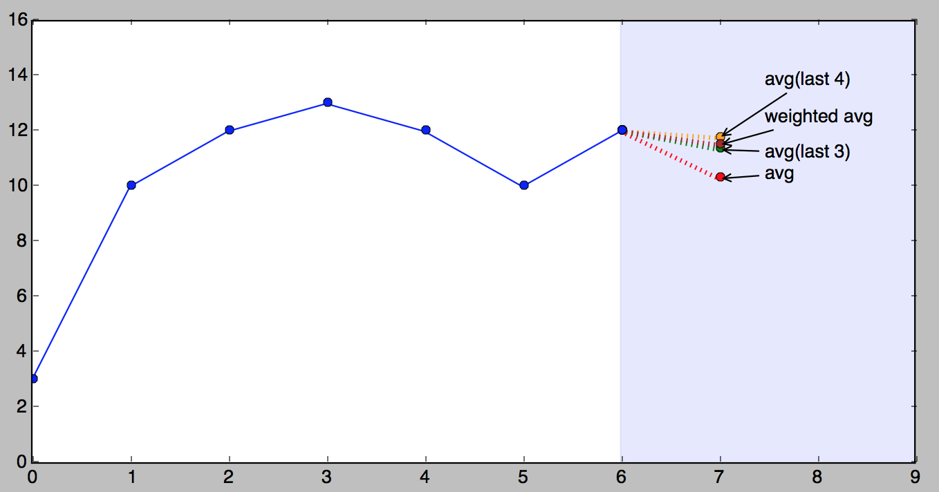
In the next few examples we are going to be using this tiny series:
1
series=[3,10,12,13,12,10,12]
(Feel free to paste it and any of the following code snippets into your Python
repl)
Naive Method
This is the most primitive forecasting method. The premise of the
naive method is that the expected point is equal to the last
observed point:
Using this method we would forecast the next point to be 12.
Simple Average
A less primitive method is the arithmetic average
of all the previously observed data points. We take all the values we
know, calculate the average and bet that that’s going to be the next value. Of course it won’t be it exactly,
but it probably will be somewhere in the ballpark, hopefully you can see the reasoning behind this
simplistic approach.
(Okay, this formula is only here because I think the capital Sigma
looks cool. I am sincerely hoping that the average requires no explanation.) In Python:
123456
defaverage(series):returnfloat(sum(series))/len(series)# Given the above series, the average is:# >>> average(series)# 10.285714285714286
As a forecasting method, there are actually situations where it’s spot
on. For example your final school grade may be the average of all the
previous grades.
Moving Average
An improvement over simple average is the average of $n$ last
points. Obviously the thinking here is that only the recent values
matter. Calculation of the moving average involves what is sometimes
called a “sliding window” of size $n$:
12345678
# moving average using n last pointsdefmoving_average(series,n):returnaverage(series[-n:])# >>> moving_average(series, 3)# 11.333333333333334# >>> moving_average(series, 4)# 11.75
A moving average can actually be quite effective, especially if you
pick the right $n$ for the series. Stock analysts adore it.
Also note that simple average is a variation of a moving average, thus
the two functions above could be re-written as a single recursive one
(just for fun):
A weighted moving average is a moving average where within the
sliding window values are given different weights, typically so that
more recent points matter more.
Instead of selecting a window size, it requires a list of weights
(which should add up to 1). For example if we picked [0.1,
0.2, 0.3, 0.4] as weights, we would be giving 10%, 20%, 30% and 40%
to the last 4 points respectively. In Python:
1234567891011
# weighted average, weights is a list of weightsdefweighted_average(series,weights):result=0.0weights.reverse()forninrange(len(weights)):result+=series[-n-1]*weights[n]returnresult# >>> weights = [0.1, 0.2, 0.3, 0.4]# >>> weighted_average(series, weights)# 11.5
Weighted moving average is fundamental to what follows, please take a
moment to understand it, give it a think before reading on.
I would also like to stress the importance of the weights adding up
to 1. To demonstrate why, let’s say we pick weights [0.9, 0.8, 0.7,
0.6] (which add up to 3.0). Watch what happens:
12
>>> weighted_average(series, [0.9, 0.8, 0.7, 0.6])
>>> 35.5  # <--- this is clearly bogus
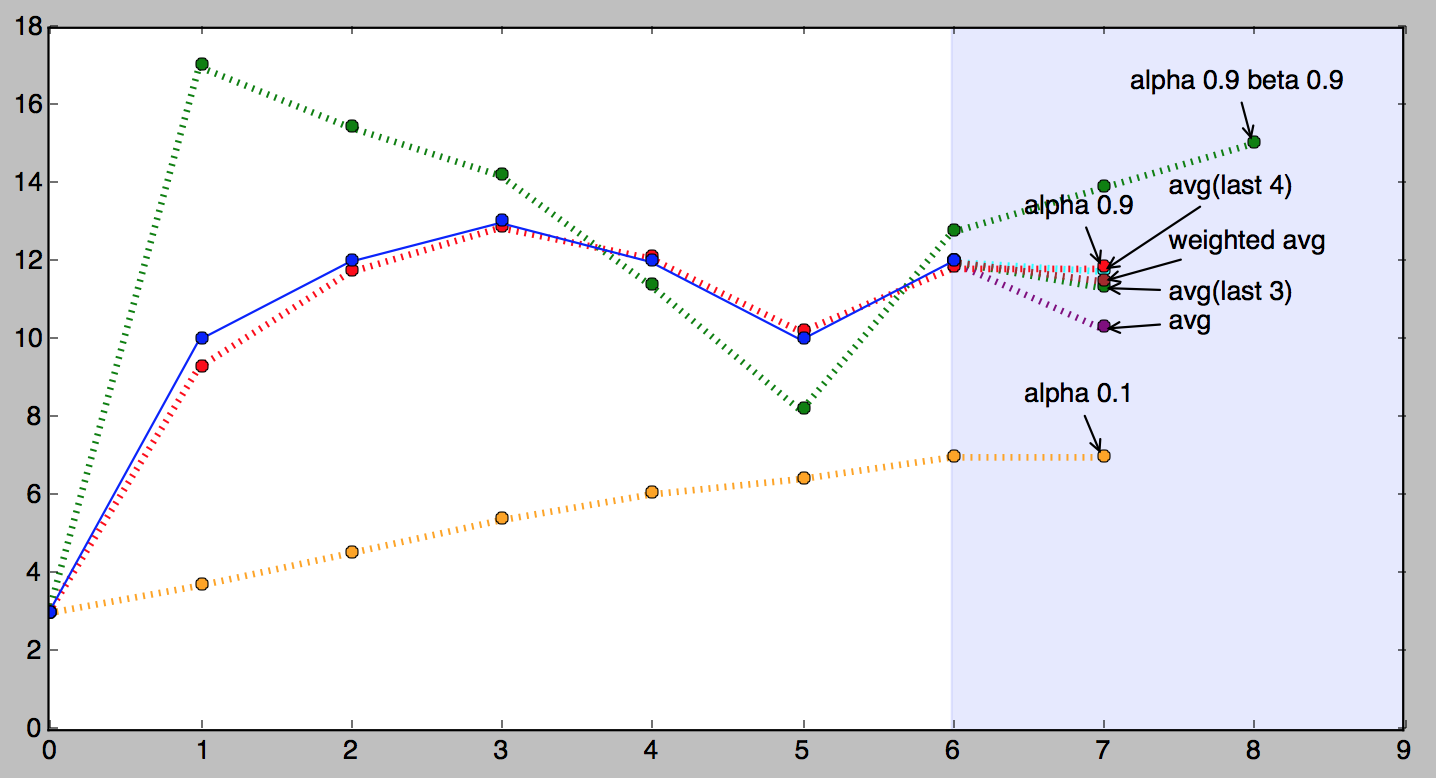
Picture time!
Here is a picture that demonstrates our tiny series and all of the above
forecasts (except for naive).
It’s important to understand that which of the above methods is better
very much depends on the nature of the series. The order in which I
presented them was from simple to complex, but “more complex” doesn’t
necessarily mean “better”.
Single Exponential Smoothing
Here is where things get interesting. Imagine a weighted average where
we consider all of the data points, while assigning exponentially
smaller weights as we go back in time. For example if we started with
0.9, our weights would be (going back in time):
…eventually approaching the big old zero. In some way this is very
similar to the weighted average above, only the weights are dictated
by math, decaying uniformly. The smaller the starting weight, the
faster it approaches zero.
Only… there is a problem: weights do not add up to 1. The sum of
the first 3 numbers alone is already 2.439! (Exercise for the reader: what number
does the sum of the weights approach and why?)
What earned Poisson, Holts or Roberts a permanent place in the history
of Mathematics is solving this with a succinct and elegant formula:
If you stare at it just long enough, you will see that the expected
value $\hat{y}_x$ is the sum of two products: $\alpha \cdot y_x$ and
$(1-\alpha) \cdot \hat{y}_{x-1}$. You can think of $\alpha$ (alpha)
as a sort of a starting weight 0.9 in the above (problematic)
example. It is called the smoothing factor or smoothing
coefficient (depending on who wrote your text book).
So essentially we’ve got a weighted moving average with two weights:
$\alpha$ and $1-\alpha$. The sum of $\alpha$ and $1-\alpha$ is 1, so
all is well.
Now let’s zoom in on the right side of the sum. Cleverly, $1-\alpha$
is multiplied by the previous expected value
$\hat{y}_{x-1}$. Which, if you think about it, is the result of the
same formula, which makes the expression recursive (and programmers
love recursion), and if you were to write it all out on paper you would
quickly see that $(1-\alpha)$ is multiplied by itself again and again
all the way to beginning of the series, if there is one, infinitely
otherwise. And this is why this method is called
exponential.
Another important thing about $\alpha$ is that its value dictates how
much weight we give the most recent observed value versus the last
expected. It’s a kind of a lever that gives more weight to the left
side when it’s higher (closer to 1) or the right side when it’s lower
(closer to 0).
Perhaps $\alpha$ would be better referred to as memory decay rate: the
higher the $\alpha$, the faster the method “forgets”.
Why is it called “smoothing”?
To the best of my understanding this simply refers to the effect these
methods have on a graph if you were to plot the values: jagged lines
become smoother. Moving average also has the same effect, so it
deserves the right to be called smoothing just as well.
Implementation
There is an aspect of this method that programmers would appreciate
that is of no concern to mathematicians: it’s simple and efficient to
implement. Here is some Python. Unlike the previous examples, this
function returns expected values for the whole series, not just one
point.
1234567891011
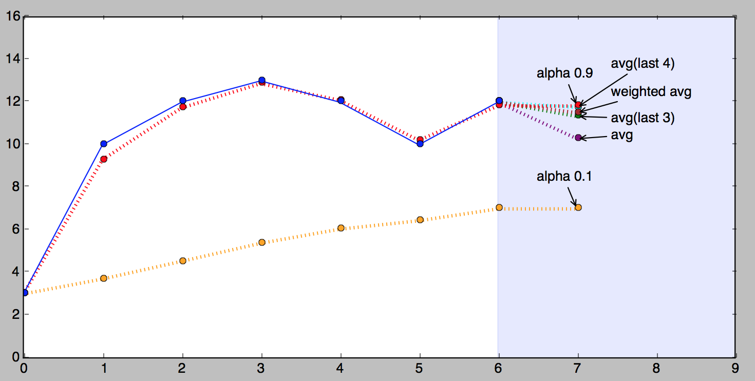
# given a series and alpha, return series of smoothed pointsdefexponential_smoothing(series,alpha):result=[series[0]]# first value is same as seriesforninrange(1,len(series)):result.append(alpha*series[n]+(1-alpha)*result[n-1])returnresult# >>> exponential_smoothing(series, 0.1)# [3, 3.7, 4.53, 5.377, 6.0393, 6.43537, 6.991833]# >>> exponential_smoothing(series, 0.9)# [3, 9.3, 11.73, 12.873000000000001, 12.0873, 10.20873, 11.820873]
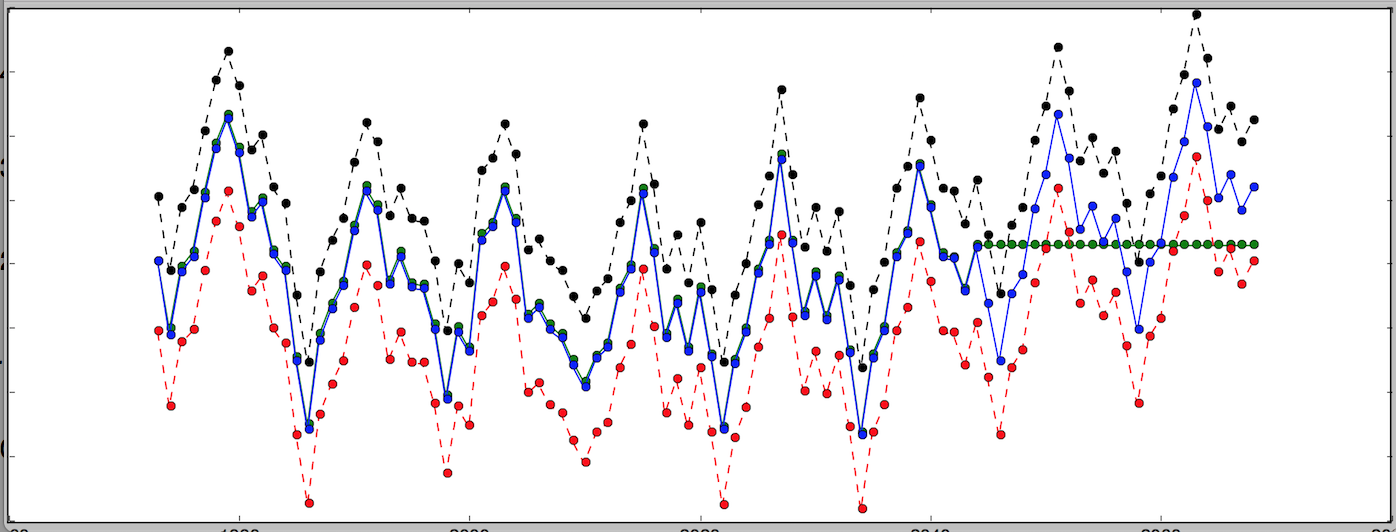
The figure below shows exponentially smoothed version of our series
with $\alpha$ of 0.9 (red) and $\alpha$ of 0.1 (orange).
Looking at the above picture it is apparent that the $\alpha$ value of 0.9
follows the observed values much closer than 0.1. This isn’t going to
be true for any series, each series has its best $\alpha$ (or
several). The process of finding the best $\alpha$ is referred to as
fitting and we will discuss it later separately.
Quick Review
We’ve learned some history, basic terminology (series and how it knows
no time, method, error SSE, MSE and fitting). And we’ve learned some
basic forecasting methods: naive, simple average, moving average,
weighted moving average and, finally, single exponential smoothing.
One very important characteristic of all of the above methods is that
remarkably, they can only forecast a single point. That’s correct,
just one.
In Part II we will focus on methods that can forecast more than
one point.
With the latest advances in PostgreSQL (and other db’s), a relational
database begins to look like a very viable TS storage platform. In
this write up I attempt to show how to store TS in PostgreSQL. (2016-12-17 Update:
there is a part 2 of this article.)
A TS is a series of [timestamp, measurement] pairs, where measurement
is typically a floating point number. These pairs (aka “data points”)
usually arrive at a high and steady rate. As time goes on, detailed
data usually becomes less interesting and is often consolidated into
larger time intervals until ultimately it is expired.
The obvious approach
The “naive” approach is a three-column table, like so:
1
CREATETABLEts(idINT,timeTIMESTAMPTZ,valueREAL);
(Let’s gloss over some details such as an index on the time column and
choice of data type for time and value as it’s not relevant to this
discussion.)
One problem with this is the inefficiency of appending data. An insert
requires a look up of the new id, locking and (usually) blocks until
the data is synced to disk. Given the TS’s “firehose” nature, the
database can quite quickly get overwhelmed.
This approach also does not address consolidation and eventual
expiration of older data points.
Round-robin database
A better alternative is something called a round-robin database. An
RRD is a circular structure with a separately stored pointer denoting
the last element and its timestamp.
A everyday life example of an RRD is a week. Imagine a structure of 7
slots, one for each day of the week. If you know today’s date and day
of the week, you can easily infer the date for each slot. For example
if today is Tuesday, April 1, 2008, then the Monday slot refers to
March 31st, Sunday to March 30th and (most notably) Wednesday to March
26.
Here’s what a 7-day RRD of average temperature might look as of
Tuesday, April 1:
Note how little has changed, and that the update required no
allocation of space: all we did to record 92F on Wednesday is
overwrite one value. Even more remarkably, the previous value
automatically “expired” when we overwrote it, thus solving the
eventual expiration problem without any additional operations.
RRD’s are also very space-efficient. In the above example we specified
the date of every slot for clarity. In an actual implementation only
the date of the last slot needs to be stored, thus the RRD can be kept
as a sequence of 7 numbers plus the position of the last entry and
it’s timestamp. In Python syntax it’d look like this:
1
[[79,82,90,92,75,80,81],2,1207022400]
Round-robin in PostgreSQL
Here is a naive approach to having a round-robin table. Carrying on
with our 7 day RRD example, it might look like this:
Somewhere separately we’d also need to record that the last entry is
week_day 3 (Tuesday) and it’s 2008-04-01. Come April 2, we could
record the temperature using:
1
UPDATEseriesSETtemp_f=92WHEREweek_day=4;
This might be okay for a 7-slot RRD, but a more typical TS might have
a slot per minute going back 90 days, which would require 129600
rows. For recording data points one at a time it might be fast enough,
but to copy the whole RRD would require 129600 UPDATE statements which
is not very efficient.
This is where using PostgrSQL arrays become very useful.
Using PostgreSQL arrays
An array would allow us to store the whole series in a single
row. Sticking with the 7-day RRD example, our table would be created
as follows:
(In PostgreSQL arrays are 1-based, not 0-based like in most
programming languages)
But it could be even more efficient
Under the hood, PostgreSQL data is stored in pages of 8K. It would
make sense to keep chunks in which our RRD is written to disk in line
with page size, or at least smaller than one page. (PostgreSQL provides
configuration parameters for how much of a page is used, etc, but this
is way beyond the scope of this article).
Having the series split into chunks also paves the way for some kind
of a caching layer, we could have a server which waits for one row
worth of data points to accumulate, then flushes then all at once.
For simplicity, let’s take the above example and expand the RRD to 4
weeks, while keeping 1 week per row. In our table definition we need
provide a way for keeping the order of every row of the TS with a
column named n, and while we’re at it, we might as well introduce a
notion of an id, so as to be able to store multiple TS in the same
table.
Let’s start with two tables, one called rrd where we would store the
last position and date, and another called ts which would store the
actual data.
The last_pos of 25 is n * 7 + 1 (since arrays are 1-based).
This article omits a lot of detail such as having resolution finer
than one day, but it does describe the general idea. For an actual
implementation of this you might want to check out a project I’ve been
working on: tgres