If you haven’t read Part I you probably should, or the following will be hard to make sense of.

All the forecasting methods we covered so far, including single exponential smoothing, were only good at predicting a single point. We can do better than that, but first we need to be introduced to a couple of new terms.

More terminology

Level

Expected value has another name, which, again varies depending on who wrote the text book: baseline, intercept (as in Y-intercept) or level. We will stick with “level” here.

So level is that one predicted point that we learned how to calculate in Part I. But because now it’s going to be only part of calculation of the forcast, we can no longer refer to it as $\hat{y}$ and will instead use $\ell$.

Trend or Slope

You should be familiar with slope from your high school algebra class. What you might be a little rusty on is how to calculate it, which is important, because a series slope has an interesting characteristic. Slope is:

where $\Delta{y}$ is the difference in the $y$ coordinates and $\Delta{x}$ is the difference in the $x$ coordinates, respectively, between two points. While in real algebraic problems $\Delta{x}$ could be anything, in a series, from one point to the next, it is always 1. Which means that for a series, slope between two adjacent points is simply $\dfrac{\Delta{y}} {1}$ or $\Delta{y}$, or:

Where $b$ is trend. To the best of my understanding terms “trend” and “slope” are interchangeable. In forecasting parlance “trend” is more common, and in math notation forecasters refer to it as $b$ rather than $m$.

Additive vs Multiplicative

Another thing to know about trend is that instead of subtracting $y_{x-1}$ from $y_x$, we could divide one by the other thereby getting a ratio. The difference between these two approaches is similar to how we can say that something costs $20 more or 5% more. The variant of the method based on subtraction is known as additive, while the one based on division is known as multiplicative.

Practice shows that a ratio (i.e. multiplicative) is a more stable predictor. The additive method, however is simpler to understand, and going from additive to multiplicative is trivial once you understand this whole thing. For this reason we will stick with the additive method here, leaving the multiplicative method an exercise for the reader.

Double Exponential Smoothing

So now we have two components to a series: level and trend. In Part I we learned several methods to forecast the level, and it should follow that every one of these methods can be applied to the trend just as well. E.g. the naive method would assume that trend between last two points is going to stay the same, or we could average all slopes between all points to get an average trend, use a moving trend average or apply exponential smoothing.

Double exponential smoothing then is nothing more than exponential smoothing applied to both level and trend. To express this in mathematical notation we now need three equations: one for level, one for the trend and one to combine the level and trend to get the expected $\hat{y}$.

The first equation is from Part I, only now we’re using $\ell$ instead of $\hat{y}$ and on the right side the expected value becomes the sum of level end trend.

The second equation introduces $\beta$, the trend factor (or coefficient). As with $\alpha$, some values of ${\beta}$ work better than others depending on the series.

Similarly to single exponential smoothing, where we used the first observed value as the first expected, we can use the first observed trend as the first expected. Of course we need at least two points to compute the initial trend.

Because we have a level and a trend, this method can forecast not one, but two data points. In Python:

1
2
3
4
5
6
7
8
9
10
11
12
13
14
15
16
17

# given a series and alpha, return series of smoothed points
def double_exponential_smoothing(series, alpha, beta):
    result = [series[0]]
    for n in range(1, len(series)+1):
        if n == 1:
            level, trend = series[0], series[1] - series[0]
        if n >= len(series): # we are forecasting
          value = result[-1]
        else:
          value = series[n]
        last_level, level = level, alpha*value + (1-alpha)*(level+trend)
        trend = beta*(level-last_level) + (1-beta)*trend
        result.append(level+trend)
    return result

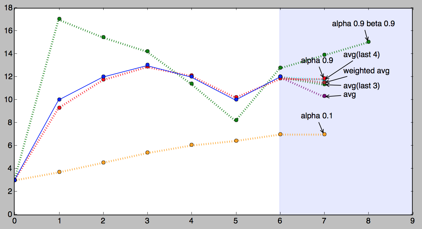
# >>> double_exponential_smoothing(series, alpha=0.9, beta=0.9)
# [3, 17.0, 15.45, 14.210500000000001, 11.396044999999999, 8.183803049999998, 12.753698384500002, 13.889016464000003]

And here is a picture of double exponential smoothing in action (the green dotted line).

Quick Review

We’ve learned that a data point in a series can be represented as a level and a trend, and we have learned how to appliy exponential smoothing to each of them to be able to forecast not one, but two points.

In Part III we’ll finally talk about triple exponential smoothing.