This three part write up [Part II Part III] is my attempt at a down-to-earth explanation (and Python code) of the Holt-Winters method for those of us who while hypothetically might be quite good at math, still try to avoid it at every opportunity. I had to dive into this subject while tinkering on tgres (which features a Golang implementation). And having found it somewhat complex (and yet so brilliantly simple), figured that it’d be good to share this knowledge, and in the process, to hopefully solidify it in my head as well.

Triple Exponential Smoothing, also known as the Holt-Winters method, is one of the many methods or algorithms that can be used to forecast data points in a series, provided that the series is “seasonal”, i.e. repetitive over some period.

A little history

Еxponential smoothing in some form or another dates back to the work of Siméon Poisson (1781-1840), while its application in forecasting appears to have been pioneered over a century later in 1956 by Robert Brown (1923–2013) in his publication Exponential Smoothing for Predicting Demand, (Cambridge, Massachusetts). [Based on the URL it seems Brown was working on forecasting tobacco demand?]

In 1957 an MIT and University of Chicago graduate, professor Charles C Holt (1921-2010) was working at CMU (then known as CIT) on forecasting trends in production, inventories and labor force. It appears that Holt and Brown worked independently and knew not of each-other’s work. Holt published a paper “Forecasting trends and seasonals by exponentially weighted moving averages” (Office of Naval Research Research Memorandum No. 52, Carnegie Institute of Technology) describing double exponential smoothing. Three years later, in 1960, a student of Holts (?) Peter R. Winters improved the algorithm by adding seasonality and published Forecasting sales by exponentially weighted moving averages (Management Science 6, 324–342), citing Dr. Holt’s 1957 paper as earlier work on the same subject. This algorithm became known as triple exponential smoothing or the Holt-Winters method, the latter probably because it was described in a 1960 Prentice-Hall book “Planning Production, Inventories, and Work Force” by Holt, Modigliani, Muth, Simon, Bonini and Winters - good luck finding a copy!

Curiously, I’ve not been able to find any personal information on Peter R. Winters online. If you find anything, please let me know, I’ll add a reference here.

In 2000 the Holt-Winters method became well known in the ISP circles at the height of the .com boom when Jake D. Brutlag (then of WebTV) published Aberrant Behavior Detection in Time Series for Network Monitoring (Proceedings of the 14th Systems Administration Conference, LISA 2000). It described how an open source C implementation [link to the actual commit] of a variant of the Holt-Winters seasonal method, which he contributed as a feature to the very popular at ISPs RRDTool, could be used to monitor network traffic.

In 2003, a remarkable 40+ years since the publication of Winters paper, professor James W Taylor of Oxford University extended the Holt-Winters method to multiple seasonalities (i.e. $n$-th exponential smoothing) and published Short-term electricity demand forecasting using double seasonal exponential smoothing (Journal of Operational Research Society, vol. 54, pp. 799–805). (But we won’t cover Taylors method here).

In 2011 the RRDTool implementation contributed by Brutlag was ported to Graphite by Matthew Graham thus making it even more popular in the devops community.

So… how does it work?

Forecasting, Baby Steps

The best way to explain triple exponential smoothing is to gradually build up to it starting with the simplest forecasting methods. Lest this text gets too long, we will stop at triple exponential smoothing, though there are quite a few other methods known.

I used mathematical notation only where I thought it made best sense, sometimes accompanied by an “English translation”, and where appropriate supplemented with a bit of Python code. In Python I refrain from using any non-standard packages, keeping the examples plain. I chose not to use generators for clarity. The objective here is to explain the inner working of the algorithm so that you can implement it yourself in whatever language you prefer.

I also hope to demonstrate that this is simple enough that you do not need to resort to SciPy or whatever (not that there is anything wrong with that).

But First, Some Terminology

Series

The main subject here is a series. In the real world we are most likely to be applying this to a time series, but for this discussion the time aspect is irrelevant. A series is merely an ordered sequence of numbers. We might be using words that are chronological in nature (past, future, yet, already, time even!), but only because it makes it easer to understand. So forget about time, timestamps, intervals, time does not exist, the only property each data point has (other than the value) is its order: first, next, previous, last, etc.

It is useful to think of a series as a list of two-dimensional $x,y$ coordinates, where $x$ is order (always going up by 1), and $y$ is value. For this reason in our math formulas we will be sticking to $y$ for value and $x$ for order.

Observed vs Expected

Forecasting is estimating values that we do not yet know based on the the values we do know. The values we know are referred to as observed while the values we forecast as expected. The math convention to denote expected values is with the circumflex a.k.a. “hat”: $\hat{y}$

For example, if we have a series that looks like [1,2,3], we might forecast the next value to be 4. Using this terminology, given observed series [1,2,3] the next expected value ${\hat{y}_4}$ is 4.

Method

We may have intuited based on [1,2,3] that in this series each value is 1 greater than the previous, which in math notation can be expressed as and $\hat{y}_{x + 1} = y_x + 1$. This equation, the result of our intuition, is known as a forecast method.

If our method is correct then the next observed value would indeed be 4, but if [1,2,3] is actually part of a Fibonacci sequence, then where we expected ${\hat{y}_4 = 4}$, we would observe $y_4 = 5$. Note the hatted ${\hat{y}}$ (expected) in the former and $y$ (observed) in the latter expression.

Error, SSE and MSE

It is perfectly normal to compute expected values where we already have observed values. Comparing the two lets you compute the error, which is the difference between observed and expected and is an indispensable indication of the accuracy of the method.

Since difference can be negative or positive, the common convention is to use the absolute value or square the error so that the number is always positive. For a whole series the squared errors are typically summed resulting in Sum of Squared Errors (SSE). Sometimes you may come across _Mean Squared Error (MSE).

And Now the Methods (where the fun begins!)

In the next few examples we are going to be using this tiny series:

series = [3,10,12,13,12,10,12]

(Feel free to paste it and any of the following code snippets into your Python repl)

Naive Method

This is the most primitive forecasting method. The premise of the naive method is that the expected point is equal to the last observed point:

$\hat{y}_{x+1} = y_x$

Using this method we would forecast the next point to be 12.

Simple Average

A less primitive method is the arithmetic average of all the previously observed data points. We take all the values we know, calculate the average and bet that that’s going to be the next value. Of course it won’t be it exactly, but it probably will be somewhere in the ballpark, hopefully you can see the reasoning behind this simplistic approach.

$\hat{y}_{x+1} = \dfrac{1}{x}\sum_{i=1}^{x}y_i$

(Okay, this formula is only here because I think the capital Sigma looks cool. I am sincerely hoping that the average requires no explanation.) In Python:

def average(series):
    return float(sum(series))/len(series)

# Given the above series, the average is:
# >>> average(series)
# 10.285714285714286

As a forecasting method, there are actually situations where it’s spot on. For example your final school grade may be the average of all the previous grades.

Moving Average

An improvement over simple average is the average of $n$ last points. Obviously the thinking here is that only the recent values matter. Calculation of the moving average involves what is sometimes called a “sliding window” of size $n$:

# moving average using n last points
def moving_average(series, n):
    return average(series[-n:])

# >>> moving_average(series, 3)
# 11.333333333333334
# >>> moving_average(series, 4)
# 11.75

A moving average can actually be quite effective, especially if you pick the right $n$ for the series. Stock analysts adore it.

Also note that simple average is a variation of a moving average, thus the two functions above could be re-written as a single recursive one (just for fun):

def average(series, n=None):
    if n is None:
        return average(series, len(series))
    return float(sum(series[-n:]))/n

# >>> average(series, 3)
# 11.333333333333334
# >>> average(series)
# 10.285714285714286

Weighted Moving Average

A weighted moving average is a moving average where within the sliding window values are given different weights, typically so that more recent points matter more.

Instead of selecting a window size, it requires a list of weights (which should add up to 1). For example if we picked [0.1, 0.2, 0.3, 0.4] as weights, we would be giving 10%, 20%, 30% and 40% to the last 4 points respectively. In Python:

# weighted average, weights is a list of weights
def weighted_average(series, weights):
    result = 0.0
    weights.reverse()
    for n in range(len(weights)):
        result += series[-n-1] * weights[n]
    return result

# >>> weights = [0.1, 0.2, 0.3, 0.4]
# >>> weighted_average(series, weights)
# 11.5

Weighted moving average is fundamental to what follows, please take a moment to understand it, give it a think before reading on.

I would also like to stress the importance of the weights adding up to 1. To demonstrate why, let’s say we pick weights [0.9, 0.8, 0.7, 0.6] (which add up to 3.0). Watch what happens:

>>> weighted_average(series, [0.9, 0.8, 0.7, 0.6])
>>> 35.5  # <--- this is clearly bogus

Picture time!

Here is a picture that demonstrates our tiny series and all of the above forecasts (except for naive).

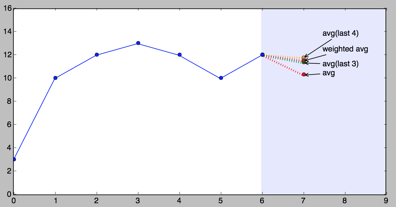
It’s important to understand that which of the above methods is better very much depends on the nature of the series. The order in which I presented them was from simple to complex, but “more complex” doesn’t necessarily mean “better”.

Single Exponential Smoothing

Here is where things get interesting. Imagine a weighted average where we consider all of the data points, while assigning exponentially smaller weights as we go back in time. For example if we started with 0.9, our weights would be (going back in time):

$0.9^1, 0.9^2, 0.9^3, 0.9^4, 0.9^5, 0.9^6... \\ \mbox{or: } 0.9, 0.81, 0.729, 0.6561, 0.59049, 0.531441, ...$

…eventually approaching the big old zero. In some way this is very similar to the weighted average above, only the weights are dictated by math, decaying uniformly. The smaller the starting weight, the faster it approaches zero.

Only… there is a problem: weights do not add up to 1. The sum of the first 3 numbers alone is already 2.439! (Exercise for the reader: what number does the sum of the weights approach and why?)

What earned Poisson, Holts or Roberts a permanent place in the history of Mathematics is solving this with a succinct and elegant formula:

$\hat{y}_x = \alpha \cdot y_x + (1-\alpha) \cdot \hat{y}_{x-1} \\$

If you stare at it just long enough, you will see that the expected value $\hat{y}_x$ is the sum of two products: $\alpha \cdot y_x$ and $(1-\alpha) \cdot \hat{y}_{x-1}$. You can think of $\alpha$ (alpha) as a sort of a starting weight 0.9 in the above (problematic) example. It is called the smoothing factor or smoothing coefficient (depending on who wrote your text book).

So essentially we’ve got a weighted moving average with two weights: $\alpha$ and $1-\alpha$. The sum of $\alpha$ and $1-\alpha$ is 1, so all is well.

Now let’s zoom in on the right side of the sum. Cleverly, $1-\alpha$ is multiplied by the previous expected value $\hat{y}_{x-1}$. Which, if you think about it, is the result of the same formula, which makes the expression recursive (and programmers love recursion), and if you were to write it all out on paper you would quickly see that $(1-\alpha)$ is multiplied by itself again and again all the way to beginning of the series, if there is one, infinitely otherwise. And this is why this method is called exponential.

Another important thing about $\alpha$ is that its value dictates how much weight we give the most recent observed value versus the last expected. It’s a kind of a lever that gives more weight to the left side when it’s higher (closer to 1) or the right side when it’s lower (closer to 0).

Perhaps $\alpha$ would be better referred to as memory decay rate: the higher the $\alpha$, the faster the method “forgets”.

Why is it called “smoothing”?

To the best of my understanding this simply refers to the effect these methods have on a graph if you were to plot the values: jagged lines become smoother. Moving average also has the same effect, so it deserves the right to be called smoothing just as well.

Implementation

There is an aspect of this method that programmers would appreciate that is of no concern to mathematicians: it’s simple and efficient to implement. Here is some Python. Unlike the previous examples, this function returns expected values for the whole series, not just one point.

# given a series and alpha, return series of smoothed points
def exponential_smoothing(series, alpha):
    result = [series[0]] # first value is same as series
    for n in range(1, len(series)):
        result.append(alpha * series[n] + (1 - alpha) * result[n-1])
    return result

# >>> exponential_smoothing(series, 0.1)
# [3, 3.7, 4.53, 5.377, 6.0393, 6.43537, 6.991833]
# >>> exponential_smoothing(series, 0.9)
# [3, 9.3, 11.73, 12.873000000000001, 12.0873, 10.20873, 11.820873]

The figure below shows exponentially smoothed version of our series with $\alpha$ of 0.9 (red) and $\alpha$ of 0.1 (orange).

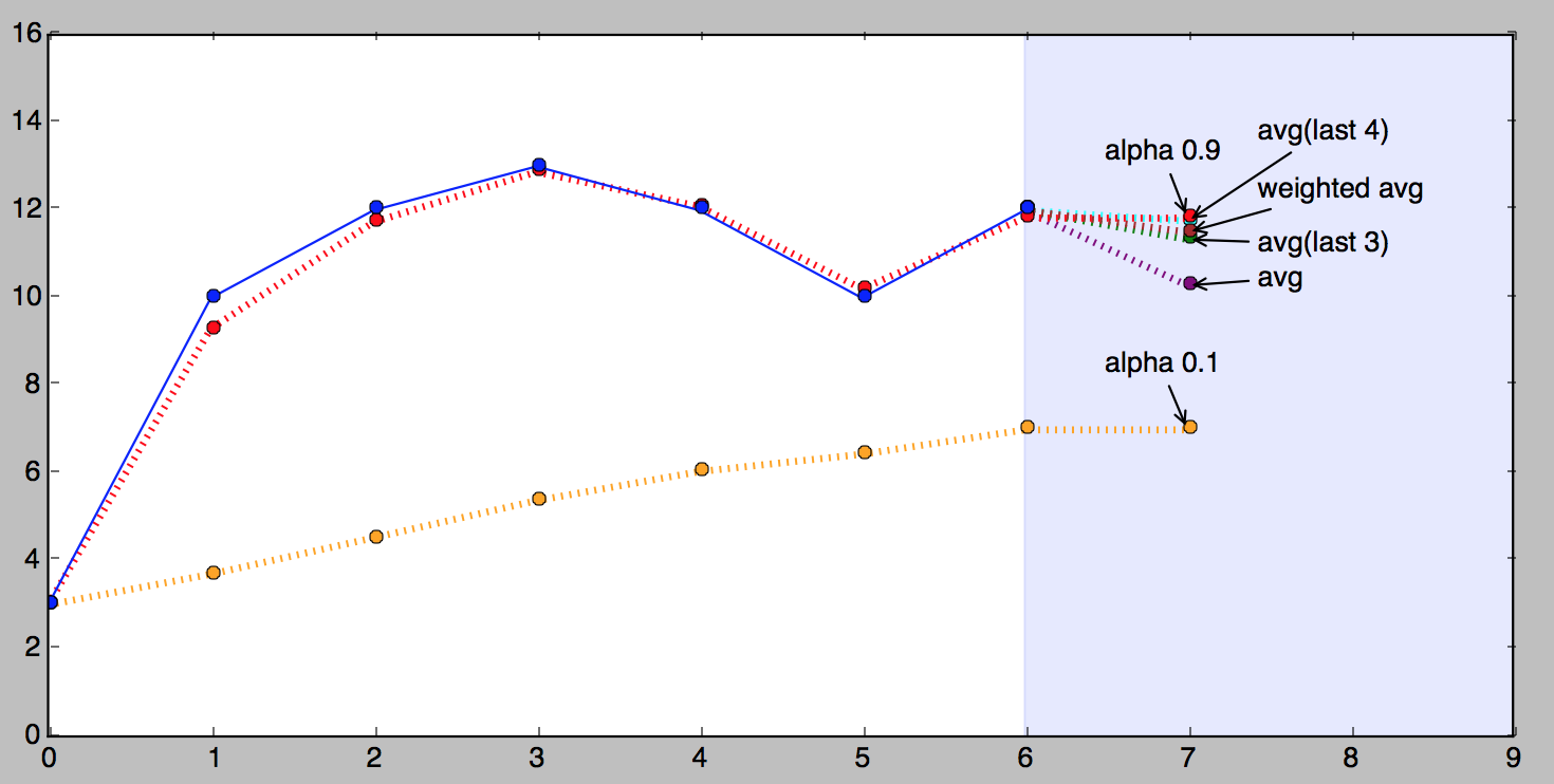
Looking at the above picture it is apparent that the $\alpha$ value of 0.9 follows the observed values much closer than 0.1. This isn’t going to be true for any series, each series has its best $\alpha$ (or several). The process of finding the best $\alpha$ is referred to as fitting and we will discuss it later separately.

Quick Review

We’ve learned some history, basic terminology (series and how it knows no time, method, error SSE, MSE and fitting). And we’ve learned some basic forecasting methods: naive, simple average, moving average, weighted moving average and, finally, single exponential smoothing.

One very important characteristic of all of the above methods is that remarkably, they can only forecast a single point. That’s correct, just one.

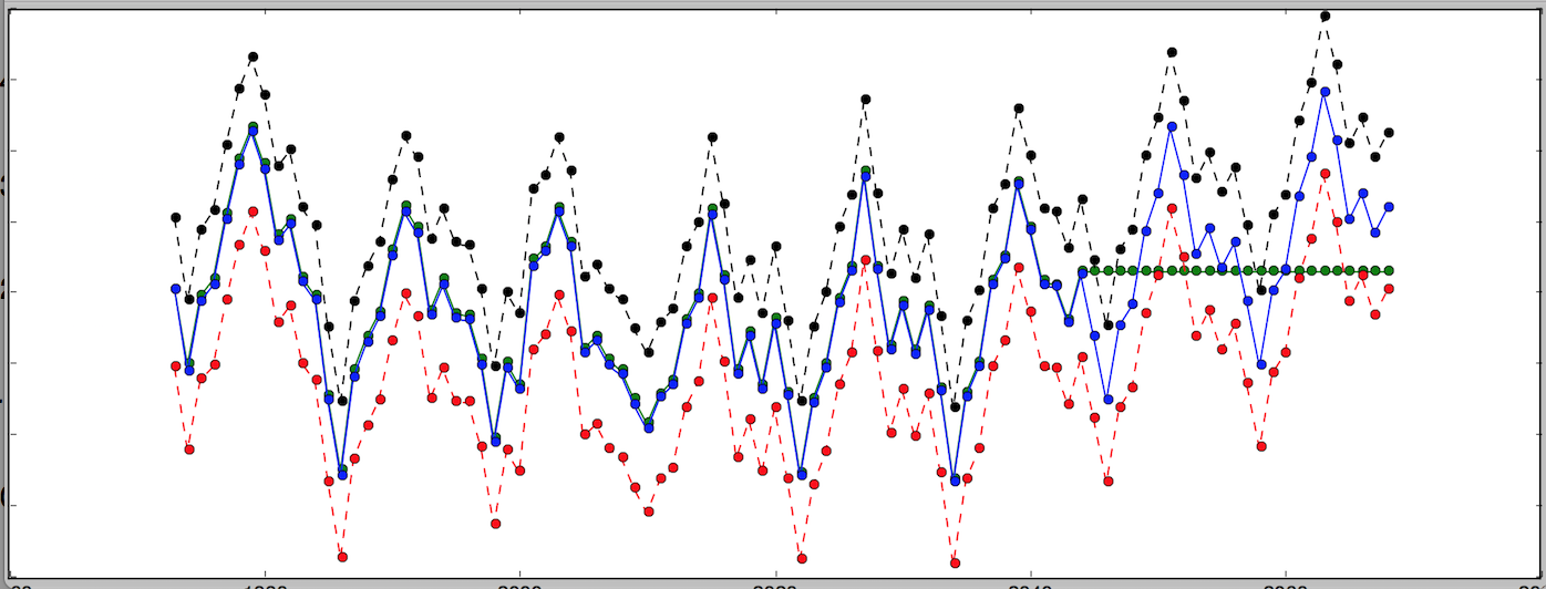
In Part II we will focus on methods that can forecast more than one point.

Gregory Trubetskoy

Notes to self.

Holt-Winters Forecasting for Dummies (or Developers) - Part I