This is a continuation of part 1. (There is also part 3 and part 4).

So our app is going to have two major parts to it: client and server. (What year is this?). The server side is going to be in Go, and the client side in JS. Let’s talk about the server side first.

The Go (Server) Side

The server side of our application is going to be responsible for initially serving up all the necessary JavaScript and supporting files if any, aka static assets and data in the form of JSON. That’s it, just two functions: (1) static assets and (2) JSON.

It’s worth noting that serving assets is optional: assets could be served from a CDN, for example. But what is different is that it is not a problem for our Go app, unlike a Python/Ruby app it can perform on par with Ngnix and Apache serving static assets. Delegating assets to another piece of software to lighten its load is no longer necessary, though certainly makes sense in some situations.

To make this simpler, let’s pretend we’re making an app that lists people (just first and last name) from a database table, that’s it. The code is here https://github.com/grisha/gowebapp.

Directory Layout

It has been my experience that dividing functionality across packages early on is a good idea in Go. Even if it is not completely clear how the final program will be structured, it is good to keep things separate to the extent possible.

For a web app I think something along the lines of the following layout makes sense:

1
2
3
4
5
6
7
8
9
10
11
12
13

# github.com/user/foo

foo/            # package main
  |
  +--daemon/    # package daemon
  |
  +--model/     # package model
  |
  +--ui/        # package ui
  |
  +--db/        # package db
  |
  +--assets/    # where we keep JS and other assets

Top level: package main

At the top level we have package main and its code in main.go. The key advantage here is that with this layout go get github.com/user/foo can be the only command required to install the whole application into $GOPATH/bin.

Package main should do as little as possible. The only code that belongs here is to parse the command argument flags. If the app had a config file, I’d stick parsing and checking of that file into yet another package, probably called config. After that main should pass the control to the daemon package.

An essential main.go is:

1
2
3
4
5
6
7
8
9
10
11
12
13
14
15
16
17
18
19
20
21
22
23
24
25
26
27
28
29
30
31
32
33

package main

import (
    "github.com/user/foo/daemon"
)

var assetsPath string

func processFlags() *daemon.Config {
    cfg := &daemon.Config{}

    flag.StringVar(&cfg.ListenSpec, "listen", "localhost:3000", "HTTP listen spec")
    flag.StringVar(&cfg.Db.ConnectString, "db-connect", "host=/var/run/postgresql dbname=gowebapp sslmode=disable", "DB Connect String")
    flag.StringVar(&assetsPath, "assets-path", "assets", "Path to assets dir")

    flag.Parse()
    return cfg
}

func setupHttpAssets(cfg *daemon.Config) {
    log.Printf("Assets served from %q.", assetsPath)
    cfg.UI.Assets = http.Dir(assetsPath)
}

func main() {
    cfg := processFlags()

    setupHttpAssets(cfg)

    if err := daemon.Run(cfg); err != nil {
        log.Printf("Error in main(): %v", err)
    }
}

The above program accepts three parameters, -listen, -db-connect and -assets-path, nothing earth shattering.

Using structs for clarity

In line cfg := &daemon.Config{} we are creating a daemon.Config object. It’s main purpose is to pass around configuration in a structured and clear format. Every one of our packages defines its own Config type describing the parameters it needs, and packages can include other package configs. We see an example of this in processFlags() above: flag.StringVar(&cfg.Db.ConnectString, .... Here db.Config is included in daemon.Config. I find doing this very useful. These structures also keep open the possibility of serializing configs as JSON, TOML or whatever.

Using http.FileSystem to serve assets

The http.Dir(assetsPath) in setupHttpAssets is in preparation to how we will serve the assets in the ui package. The reason it’s done this way is to leave the door open for cfg.UI.Assets (which is a http.FileSystem interface) to be provided by other implementations, e.g. serving this content from memory. I will describe it in more detail in a later post.

Lastly, main calls daemon.Run(cfg) which is what actually starts our app and where it blocks until it’s terminated.

package daemon

Package daemon contains everything related to running a process. Stuff like which port to listen on, custom logging would belong here, as well anything related to a graceful restart, etc.

Since the job of the daemon package is to initiate the database connection, it will need to import the db package. It’s also responsible for listening on the TCP port and starting the user interface for that listener, therefore it needs to import the ui package, and since the ui package needs to access data, which is done via the model package, it will need to import model as well.

A bare bones daemon might look like this:

1
2
3
4
5
6
7
8
9
10
11
12
13
14
15
16
17
18
19
20
21
22
23
24
25
26
27
28
29
30
31
32
33
34
35
36
37
38
39
40
41
42
43
44
45
46
47
48
49
50
51

package daemon

import (
    "log"
    "net"
    "os"
    "os/signal"
    "syscall"

    "github.com/grisha/gowebapp/db"
    "github.com/grisha/gowebapp/model"
    "github.com/grisha/gowebapp/ui"
)

type Config struct {
    ListenSpec string

    Db db.Config
    UI ui.Config
}

func Run(cfg *Config) error {
    log.Printf("Starting, HTTP on: %s\n", cfg.ListenSpec)

    db, err := db.InitDb(cfg.Db)
    if err != nil {
        log.Printf("Error initializing database: %v\n", err)
        return err
    }

    m := model.New(db)

    l, err := net.Listen("tcp", cfg.ListenSpec)
    if err != nil {
        log.Printf("Error creating listener: %v\n", err)
        return err
    }

    ui.Start(cfg.UI, m, l)

    waitForSignal()

    return nil
}

func waitForSignal() {
    ch := make(chan os.Signal)
    signal.Notify(ch, syscall.SIGINT, syscall.SIGTERM)
    s := <-ch
    log.Printf("Got signal: %v, exiting.", s)
}

Note how Config includes db.Config and ui.Config as I described earlier.

All the action happens in Run(*Config). We initialize a database connection, create a model.Model instance, and start the ui passing in the config, a pointer to the model and the listener.

package model

The purpose of model is to separate how data is stored in the database from the ui, as well as to contain any business logic an app might have. It’s the brains of the app if you will.

The model package should define a struct (Model seems like an appropriate name) and a pointer to an instance of the struct should be passed to all the ui functions and methods. There should only be one such instance in our app - for extra credit you can enforce that programmatically by making it a singleton, but I don’t think that’s necessary.

Alternatively you could get by without a Model and just use the package model itself. I don’t like this approach, but it’s an option.

The model should also define structs for the data entities we are dealing with. In our example it would be a Person struct. Its members should be exported (capitalized) because other packages will be accessing those. If you use sqlx, this is where you would also specify tags that map elements to db column names, e.g. `db:"first_name"`

Our Person type:

1
2
3
4

type Person struct {
    Id          int64
    First, Last string
}

In our case we do not need tags because our column names match the element names, and sqlx conveniently takes care of the capitalization, so Last matches the column named last.

package model should NOT import db

Somewhat counter-intuitive, model cannot import db. This is because db needs to import model, and circular imports are not allowed in Go. This is one case where interfaces come in handy. model needs to define an interface which db should satisfy. For now all we know is we need to list people, so we can start with this definition:

1
2
3

type db interface {
    SelectPeople() ([]*Person, error)
}

Our app doesn’t really do much, but we know it lists people, so our model should probably have a People() ([]*Person, error) method:

1
2
3

func (m *Model) People() ([]*Person, error) {
    return m.SelectPeople()
}

To keep things tidy, code should be in separate files, e.g. Person definition should be in person.go, etc. For readability, here is a single file version of our model:

1
2
3
4
5
6
7
8
9
10
11
12
13
14
15
16
17
18
19
20
21
22
23
24

package model

type db interface {
    SelectPeople() ([]*Person, error)
}

type Model struct {
    db
}

func New(db db) *Model {
    return &Model{
        db: db,
    }
}

func (m *Model) People() ([]*Person, error) {
    return m.SelectPeople()
}

type Person struct {
    Id          int64
    First, Last string
}

package db

db is the actual implementation of the database interaction. This is where the SQL statements are constructed and executed. This package also imports model because it will need to construct those structs from database data.

First, db needs to provide the InitDb function which will establish the database connection, as well as create the necessary tables and prepare the SQL statements.

Our simplistic example doesn’t support migrations, but in theory this is also where they might potentially happen.

We are using PostgreSQL, which means we need to import the pq driver. We are also going to rely on sqlx, and we need our own model. Here is the beginning of our db implementation:

1
2
3
4
5
6
7
8
9
10
11
12
13
14
15
16
17
18
19
20
21
22
23
24
25
26
27
28
29
30
31

package db

import (
    "database/sql"

    "github.com/grisha/gowebapp/model"
    "github.com/jmoiron/sqlx"
    _ "github.com/lib/pq"
)

type Config struct {
    ConnectString string
}

func InitDb(cfg Config) (*pgDb, error) {
    if dbConn, err := sqlx.Connect("postgres", cfg.ConnectString); err != nil {
        return nil, err
    } else {
        p := &pgDb{dbConn: dbConn}
        if err := p.dbConn.Ping(); err != nil {
            return nil, err
        }
        if err := p.createTablesIfNotExist(); err != nil {
            return nil, err
        }
        if err := p.prepareSqlStatements(); err != nil {
            return nil, err
        }
        return p, nil
    }
}

Our InitDb() creates an instance of a pgDb, which is our Postgres implementation of the model.db interface. It keeps all that we need to communicate with the database, including the prepared statements, and exports the necessary methods to satisfy the interface.

1
2
3
4
5

type pgDb struct {
    dbConn *sqlx.DB

    sqlSelectPeople *sqlx.Stmt
}

Here is the code to create the tables and the statements. From the SQL perspective this is rather simplistic, it could be a lot more elaborate, of course:

1
2
3
4
5
6
7
8
9
10
11
12
13
14
15
16
17
18
19
20
21
22
23
24
25
26
27

func (p *pgDb) createTablesIfNotExist() error {
    create_sql := `

       CREATE TABLE IF NOT EXISTS people (
       id SERIAL NOT NULL PRIMARY KEY,
       first TEXT NOT NULL,
       last TEXT NOT NULL);

    `
    if rows, err := p.dbConn.Query(create_sql); err != nil {
        return err
    } else {
        rows.Close()
    }
    return nil
}

func (p *pgDb) prepareSqlStatements() (err error) {

    if p.sqlSelectPeople, err = p.dbConn.Preparex(
        "SELECT id, first, last FROM people",
    ); err != nil {
        return err
    }

    return nil
}

Finally, we need to provide the method to satisfy the interface:

1
2
3
4
5

    people := make([]*model.Person, 0)
    if err := p.sqlSelectPeople.Select(&people); err != nil {
        return nil, err
    }
    return people, nil

Here we’re taking advantage of sqlx to run the query and construct a slice from results with a simple call to Select() (NB: p.sqlSelectPeople is a *sqlx.Stmt). Without sqlx we would have to iterate over the result rows, processing each with Scan, which would be considerably more verbose.

Beware of a very subtle “gotcha” here. people could also be defined as var people []*model.Person and the method would work just the same. However, if the database returned no rows, the method would return nil, not an empty slice. If the result of this method is later encoded as JSON, the former would become null and the latter []. This could cause problems if the client side doesn’t know how to treat null.

That’s it for db.

package ui

Finally, we need to serve all that stuff via HTTP and that’s what the ui package does.

Here is a very simplistic variant:

1
2
3
4
5
6
7
8
9
10
11
12
13
14
15
16
17
18
19
20
21
22
23
24
25
26
27
28
29
30
31
32
33
34
35
36
37
38
39
40
41
42
43
44
45

package ui

import (
    "fmt"
    "net"
    "net/http"
    "time"

    "github.com/grisha/gowebapp/model"
)

type Config struct {
    Assets http.FileSystem
}

func Start(cfg Config, m *model.Model, listener net.Listener) {

    server := &http.Server{
        ReadTimeout:    60 * time.Second,
        WriteTimeout:   60 * time.Second,
        MaxHeaderBytes: 1 << 16}

    http.Handle("/", indexHandler(m))

    go server.Serve(listener)
}

const indexHTML = `
<!DOCTYPE HTML>
<html>
  <head>
    <meta charset="utf-8">
    <title>Simple Go Web App</title>
  </head>
  <body>
    <div id='root'></div>
  </body>
</html>
`

func indexHandler(m *model.Model) http.Handler {
    return http.HandlerFunc(func(w http.ResponseWriter, r *http.Request) {
        fmt.Fprintf(w, indexHTML)
    })
}

Note how indexHTML contains next to nothing. This is 100% of the HTML that this app will ever serve. It will evolve a little as we get into the client side of the app, but only by a few lines.

Also noteworthy is how the handler is defined. If this idiom is not familiar, it’s worth spending a few minutes (or a day) to internalize it completely as it is very common in Go. indexHandler() is not a handler, it returns a handler function. It is done this way so that we can pass in a *model.Model via closure, since an HTTP handler function definition is fixed and a model pointer is not one of the parameters.

In the case of indexHandler() we’re not actually doing anything with the model pointer, but when we get to implementing an actual list of people we will need it.

Conclusion

Above is essentially all the knowledge required to build a basic Go web app, at least the Go side of it. Next week I’ll get into the client side and we will complete the people listing code.

Continue to part 3.

This is part 3. See part 1 and part 2.

The previous two posts got us to a point where we had a Go app which was able to serve a tiny bit of HTML. This post will talk about the client side, which, alas, is mostly JavaScript, not Go.

JavaScript in 2017

This is what gave me the most grief. I don’t really know how to categorize the mess that present day JavaScript is, nor do I really know what to attribute it to, and trying to rationalize it would make for a great, but entirely different blog post. So I’m just going to accept this as the reality we cannot change and move on to how to best work with it.

Variants of JS

The most common variant of JS these days is known as ES2015 (aka ES6 or ECMAScript 6th Edition), and it is mostly supported by the more or less latest browsers. The latest released spec of JavaScript is ES7 (aka ES2016), but since the browsers are sill catching up with ES6, it looks like ES7 is never really going to be adopted as such, because most likely the next coming ES8 which might be released in 2017 will supersede it before the browsers are ready.

Curiously, there appears to be no simple way to construct an environment fully specific to a particular ECMAScript version. There is not even a way to revert to an older fully supported version ES5 or ES4, and thus it is not really possible to test your script for compliance. The best you can do is to test it on the browsers you have access to and hope for the best.

Because of the ever changing and vastly varying support for the language across platforms and browsers, transpilation has emerged as a common idiom to address this. Transpilation mostly amounts to JavaScript code being converted to JavaScript that complies with a specific ES version or a particular environment. For example import Bar from 'foo'; might become var Bar = require('foo');. And so if a particular feature is not supported, it can be made available with the help of the right plug-in or transpiler. I suspect that the transpilation proliferation phenomenon has led to additional problems, such as the input expected by a transpiler assuming existence of a feature that is no longer supported, same with output. Often this might be remedied by additional plugins, and it can be very difficult to sort out. On more than one occasion I spent a lot of time trying to get something to work only to find out later that my entire approach has been obsoleted by a new and better solution now built-in to some other tool.

JS Frameworks

There also seems to be a lot of disagreement on which JS framework is best. It is even more confusing because the same framework can be so radically different from one version to the next I wonder why they didn’t just change the name.

I have no idea which is best, and I only had the patience to try a couple. About a year ago I spent a bunch of time tinkering with AngularJS, and this time, for a change, I tinkered with React. For me, I think React makes more sense, and so this is what this example app is using, for better or worse.

React and JSX

If you don’t know what React is, here’s my (technically incorrect) explanation: it’s HTML embedded in JavaScript. We’re all so brainwashed into JavaScript being embedded in HTML as the natural order of things, that inverting this relationship does not even occur as a possibility. For the fundamental simplicity of this revolutionary (sic) concept I think React is quite brilliant.

A react “Hello World!” looks approximately like this:

1
2
3
4
5
6
7
8

class Hello extends React.Component {
  render() {
    let who = "World";
    return (
      <h1> Hello {who}! </h1>
    );
  }
}

Notice how the HTML just begins without any escape or delimiter. Surprisingly, the opening “<” works quite reliably as the marker signifying beginning of HTML. Once inside HTML, the opening curly brace indicates that we’re back to JavaScript temporarily, and this is how variable values are interpolated inside HTML. That’s pretty much all you need to know to “get” React.

Technically, the above file format is known as JSX, while React is the library which provides the classes used to construct React objects such as React.Component above. JSX is transpiled into regular JavaScript by a tool known as Babel, and in fact JSX is not even required, a React component can be written in plain JavaScript, and there is a school of thought whereby React is used without JSX. I personally find the JSX-less approach a little too noisy, and I also like that Babel allows you to use a more modern dialect of JS (though not having to deal with a transpiler is definitely a win).

Minimal Working Example

First, we need three pieces of external JavaScript. They are (1) React and ReactDOM, (2) Babel in-browser transpiler and (3) a little lib called Axios which is useful for making JSON HTTP requests. I get them out of Cloudflare CDN, there are probably other ways. To do this, we need to augment our indexHTML variable to look like this:

1
2
3
4
5
6
7
8
9
10
11
12
13
14
15
16
17
18
19
20
21
22
23
24

const (
	cdnReact           = "https://cdnjs.cloudflare.com/ajax/libs/react/15.5.4/react.min.js"
	cdnReactDom        = "https://cdnjs.cloudflare.com/ajax/libs/react/15.5.4/react-dom.min.js"
	cdnBabelStandalone = "https://cdnjs.cloudflare.com/ajax/libs/babel-standalone/6.24.0/babel.min.js"
	cdnAxios           = "https://cdnjs.cloudflare.com/ajax/libs/axios/0.16.1/axios.min.js"
)

const indexHTML = `
<!DOCTYPE HTML>
<html>
  <head>
    <meta charset="utf-8">
    <title>Simple Go Web App</title>
  </head>
  <body>
    <div id='root'></div>
    <script src="` + cdnReact + `"></script>
    <script src="` + cdnReactDom + `"></script>
    <script src="` + cdnBabelStandalone + `"></script>
    <script src="` + cdnAxios + `"></script>
    <script src="/js/app.jsx" type="text/babel"></script>
  </body>
</html>
`

At the very end it now loads "/js/app.jsx" which we need to accommodate as well. Back in part 1 we created a UI config variable called cfg.Assets using http.Dir(). We now need to wrap it in a handler which serves files, and Go conveniently provides one:

1

    http.Handle("/js/", http.FileServer(cfg.Assets))

With the above, all the files in "assets/js" become available under "/js/".

Finally we need to create the assets/js/app.jsx file itself:

1
2
3
4
5
6
7
8
9
10

class Hello extends React.Component {
  render() {
    let who = "World";
    return (
      <h1> Hello {who}! </h1>
    );
  }
}

ReactDOM.render( <Hello/>, document.querySelector("#root"));

The only difference from the previous listing is the very last line, which is what makes the app actually render itself.

If we now hit the index page from a (JS-capable) browser, we should see a “Hello World”.

What happened was that the browser loaded “app.jsx” as it was instructed, but since “jsx” is not a file type it is familiar with, it simply ignored it. When Babel got its chance to run, it scanned our document for any script tags referencing “text/babel” as its type, and re-requested those pages (which makes them show up twice in developer tools, but the second request ought to served entirely from browser cache). It then transpiled it to valid JavaScript and executed it, which in turn caused React to actually render the “Hello World”.

Listing People

We need to first go back to the server side and create a URI that lists people. In order for that to happen, we need an http handler, which might look like this:

1
2
3
4
5
6
7
8
9
10
11
12
13
14
15
16
17

func peopleHandler(m *model.Model) http.Handler {
	return http.HandlerFunc(func(w http.ResponseWriter, r *http.Request) {
		people, err := m.People()
		if err != nil {
			http.Error(w, "This is an error", http.StatusBadRequest)
			return
		}

		js, err := json.Marshal(people)
		if err != nil {
			http.Error(w, "This is an error", http.StatusBadRequest)
			return
		}

		fmt.Fprintf(w, string(js))
	})
}

And we need to register it:

1

    http.Handle("/people", peopleHandler(m))

Now if we hit "/people", we should get a "[]" in response. If we insert a record into our people table with something along the lines of:

1

INSERT INTO people (first, last) VALUES('John', 'Doe');

The response should change to [{"Id":1,"First":"John","Last":"Doe"}].

Finally we need to hook up our React/JSX code to make it all render.

For this we are going to create a PersonItem component, and another one called PeopleList which will use PersonItem.

A PersonItem only needs to know how to render itself as a table row:

1
2
3
4
5
6
7
8
9
10
11

class PersonItem extends React.Component {
  render() {
    return (
      <tr>
        <td> {this.props.id}    </td>
        <td> {this.props.first} </td>
        <td> {this.props.last}  </td>
      </tr>
    );
  }
}

A PeopleList is slightly more complicated:

1
2
3
4
5
6
7
8
9
10
11
12
13
14
15
16
17
18
19
20
21
22
23
24
25
26
27
28
29
30
31
32
33

class PeopleList extends React.Component {
  constructor(props) {
    super(props);
    this.state = { people: [] };
  }

  componentDidMount() {
    this.serverRequest =
      axios
        .get("/people")
        .then((result) => {
           this.setState({ people: result.data });
        });
  }

  render() {
    const people = this.state.people.map((person, i) => {
      return (
        <PersonItem key={i} id={person.Id} first={person.First} last={person.Last} />
      );
    });

    return (
      <div>
        <table><tbody>
          <tr><th>Id</th><th>First</th><th>Last</th></tr>
          {people}
        </tbody></table>

      </div>
    );
  }
}

It has a constructor which initializes a this.state variable. It also declared a componentDidMount() method, which React will call when the component is about to be rendered, making it the (or one of) correct place to fetch the data from the server. It fetches the data via an Axios call, and saves the result in this.state.people. Finally, render() iterates over the contents of this.state.people creating an instance of PersonItem for each.

That’s it, our app now responds with a (rather ugly) table listing people from our database.

Conclusion

In essence, this is all you need to know to make a fully functional Web App in Go. This app has a number of shortcomings, which I will hopefully address later. For example in-browser transpilation is not ideal, though it might be fine for a low volume internal app where page load time is not important, so we might want to have a way to pre-transpile it ahead of time. Also our JSX is confined to a single file, this might get hard to manage for any serious size app where there are lots of components. The app has no navigation. There is no styling. There are probably things I’m forgetting about…

Enjoy!

P.S. Complete code is here

Continued in part 4…

This is part 4. See part 1, part 2 and part 3.

In this part I will try to briefly go over the missing pieces in our very simplistic Go Web App.

HTTP Handler Wrappers

I tiny rant: I do not like the word “middleware”. The concept of a wrapper has been around since the dawn of computing, there is no need to invent new words for it.

Having that out of the way, let’s say we need to require authentication for a certain URL. This is what our index handler presently looks like:

1
2
3
4
5

func indexHandler(m *model.Model) http.Handler {
	return http.HandlerFunc(func(w http.ResponseWriter, r *http.Request) {
		fmt.Fprintf(w, indexHTML)
	})
}

We could write a function which takes an http.Handler as an argument and returns a (different) http.Handler. The returned handler checks whether the user is authenticated with m.IsAuthenticated() (whatever it does is not important here) and redirects the user to a login page, or executes the original handler by calling its ServeHTTP() method.

1
2
3
4
5
6
7
8
9

func requireLogin(h http.Handler, m *model.Model) http.Handler {
	return http.HandlerFunc(func(w http.ResponseWriter, r *http.Request) {
		if !m.IsAuthenticated(r) {
			http.Redirect(w, r, loginURL, http.StatusFound)
			return
		}
		h.ServeHTTP(w, r)
	})
}

Given the above, the function registration now would look like this:

1

   http.Handle("/", requireLogin(indexHandler(m)), m)

Handlers can be wrapped this way in as many layers as needed and this approach is very flexible. Anything from setting headers to compressing output can be accomplished via a wrapper. Note also that we can pass in whatever arguments we need, for example our *model.Model.

URL Parameters

Sooner or later we might want to rely on URL parameters, e.g. /person/3 where 3 is a person id. Go standard library doesn’t provide any support for this leaving it as an exercise for the developer. The software component responsible for this sort of thing is known as a Mux or “router” and it can be replaced by a custom implementation. A Mux also provides a ServeHTTP() method which means it satisfies the http.Handler interface, i.e. it is a handler.

A very popular implementation is the Gorilla Mux. It is easy to delegate entire sub-urls to the Gorilla Mux wherever more flexibility is needed. For example we can decide that everything from /person and below is handled by an instance of a Gorilla router and we want that to be all authenticated, which might look like this:

1
2
3
4
5
6

	// import "github.com/gorilla/mux"
	pr := mux.NewRouter().PathPrefix("/person").Subrouter()
	pr.Handle("/{id}", personGetHandler(m)).Methods("GET")
	pr.Handle("/", personPostHandler(m)).Methods("POST")
	pr.Handle("/{id}", personPutHandler(m)).Methods("PUT")
	http.Handle("/person/", requireLogin(pr))

NB: I found that trailing slashes are important and the rules on when they are required are a bit confusing.

There are many other router/mux implementations out there, the beauty of not buying into any kind of a framework is that we can choose the one that works best for us or write our own (they are not difficult to implement).

Asset Handling

One of the neatest things about Go is that a compiled program is a single binary not a big pile of files like it is with most scripting languages and even compiled ones. But if our program relies on assets (JS, CSS, image and other files), we would need to copy those over to the server at deployment time.

There is a way we can preserve the “one binary” characteristic of our program by including assets as part of the binary itself. For that there is the go-bindata project and its nephew go-bindata-assetfs.

Since packing assets into the binary is slightly beyond what go build can accomplish, we will need some kind of a script to take care of it. My personal preference is to use the tried and true make, and it is not uncommon to see Go projects come with a Makefile.

Here is a relevant example Makefile rule

1
2
3
4
5
6

ASSETS_DIR = "assets"
build:
	@export GOPATH=$${GOPATH-~/go} && \
	go get github.com/jteeuwen/go-bindata/... github.com/elazarl/go-bindata-assetfs/... && \
	$$GOPATH/bin/go-bindata -o bindata.go -tags builtinassets ${ASSETS_DIR}/... && \
	go build -tags builtinassets -ldflags "-X main.builtinAssets=${ASSETS_DIR}"

The above rule creates a bindata.go file which will be placed in the same directory where main.go is and becomes part of package main. main.go will somehow know that assets are built-in and this is accomplished via an -ldflags "-X main.builtinAssets=${ASSETS_DIR}" trick, which is a way to assign values to variables at compile time. This means that our code can now check for the value of builtinAssets to decide what to do, e.g.:

1
2
3
4
5
6
7

	if builtinAssets != "" {
		log.Printf("Running with builtin assets.")
		cfg.UI.Assets = &assetfs.AssetFS{Asset: Asset, AssetDir: AssetDir, AssetInfo: AssetInfo, Prefix: builtinAssets}
	} else {
		log.Printf("Assets served from %q.", assetsPath)
		cfg.UI.Assets = http.Dir(assetsPath)
	}

The second important thing is that we are defining a build tag called builtinassets. We are also telling go-bindata about it, what this means is “only compile me when builtinassets is set”, and this controls under which circumstances bindata.go (which contains our assets as Go code) is to actually be compiled.

Pre-transpilation of JavaScript

Last, but not the least, I want to briefly mention packing of web assets. To describe it properly is enough material for a whole new series of posts, and this would really have nothing to do with Go. But I can at least list the following points.

• You might as well give in and install npm, and make a package.json file.

• Once npm is installed, it is trivial to install the Babel command-line compiler, babel-cli, which is one way to transpile JavaScript.

• A more complicated, frustrating, but ultimately more flexible method is to use webpack. Webpack will pre-transpile and do things like combine all JS into a single file as well as minimize it.

• I was surprised by how difficult it was to provide module import functionality in JavaScript. The problem is that there is an ES6 standard for import and export keywords, but there is no implementation, and even Babel assumes that something else implements it for you. In the end I settled on SystemJS. The complication with SystemJS is that now in-browser Babel transpilation needs to be something that SystemJS is aware of, so I had to use its Babel plugin for that. Webpack in turn (I think?) provides its own module support implementation, so SystemJS is not needed when assets are packed. Anyhow, it was all rather frustrating.

Conclusion

I would say that in the set up I describe in this four part series Go absolutely shines, while JavaScript not so much. But once I got over the initial hurdle of getting it all to work, React/JSX was easy and perhaps even pleasant to work with.

That’s it for now, hope you find this useful.

After nearly two years of hacking, I am tagging this version of Tgres as beta. It is functional and stable enough for people to try out and not feel like they are wasting their time. There is still a lot that could and should be improved, but at this point the most important thing is to get more people to check it out.

What is Tgres?

Tgres is a Go program which can receive time series data via Graphite, Statsd protocols or an http pixel, store it in PostgreSQL, and provide Graphite-like access to the data in a way that is compatible with tools such as Grafana. You could think of it as a drop-in Graphite/Statsd replacement, though I’d rather avoid direct comparison, because the key feature of Tgres is that data is stored in PostgreSQL.

Why PostgreSQL?

The “grand vision” for Tgres begins with the database. Relational databases have the most man-decades of any storage type invested into them, and PostgreSQL is probably the most advanced implementation presently in existence.

If you search for “relational databases and time series” (or some variation thereupon), you will come across the whole gamut of opinions (if not convictions) varying so widely it is but discouraging. This is because time series storage, while simple at first glance, is actually fraught with subtleties and ambiguities that can drive even the most patient of us up the wall.

Avoid Solving the Storage Problem.

Someone once said that “anything is possible when you don’t know what you’re talking about”, and nowhere is it more evident than in data storage. File systems and relational databases trace their origin back to the late 1960s and over half a century later I doubt that any field experts would say “the storage problem is solved”. And so it seems almost foolish to suppose that by throwing together a key-value store and a concensus algorithm or some such it is possible to come up with something better? Instead of re-inventing storage, why not focus on how to structure the data in a way that is compatible with a storage implementation that we know works and scales reliably?

As part of the Tgres project, I thought it’d be interesting to get to the bottom of this. If not bottom, then at least deeper than most people dare to dive. I am not a mathematician or a statistician, nor am I a data scientist, whatever that means, but I think I understand enough about the various subjects involved, including programming, that I can come up with something more than just another off-the-cuff opinion.

And so now I think I can conclude definitively that time series data can be stored in a relational database very efficently, PostgreSQL in particular for its support for arrays. The general approach I described in a series of blogs starting with this one, Tgres uses the technique described in the last one. In my performance tests the Tgres/Postgres combination was so efficient it was possibly outperforming its time-series siblings.

The good news is that as a user you don’t need to think about the complexities of the data layout, Tgres takes care of it. Still I very much wish people would take more time to think about how to organize data in a tried and true solution like PostgreSQL before jumping ship into the murky waters of the “noSQL” ocean, lured by alternative storage sirens, big on promise but shy on delivery, only to drown where no one could come to the rescue.

How else is Tgres different?

Tgres is a single program, a single binary which does everything (one of my favorite things about Go). It supports all of Graphite and Statsd protocols without having to run separate processes, there are no dependencies of any kind other than a PostgreSQL database. No need for Python, Node or a JVM, just the binary, the config file and access to a database.

And since the data is stored in Postgres, virtually all of the features of Postgres are available: from being able to query the data using real SQL with all the latest features, to replication, security, performance, back-ups and whatever else Postgres offers.

Another benefit of data being in a database is that it can be accessible to any application frameworks in Python, Ruby or whatever other language as just another database table. For example in Rails it might be as trivial as class Tv < ActiveRecord::Base; end et voilà, you have the data points as a model.

It should also be mentioned that Tgres requires no PostgreSQL extensions. This is because optimizing by implementing a custom extension which circumvents the PostgreSQL natural way of handling data means we are solving the storage problem again. PostgreSQL storage is not broken to begin with, no customization is necessary to handle time series.

In addition to being a standalone program, Tgres packages aim to be useful on their own as part of any other Go program. For example it is very easy to equip a Go application with Graphite capabilities by providing it access to a database and using the provided http handler. This also means that you can use a separate Tgres instance dedicated to querying data (perhaps from a downstream Potgres slave).

Some Internals Overview

Internally, Tgres series identification is tag-based. The series are identified by a JSONB field which is a set of key/value pairs indexed using a GIN index. In Go, the JSONB field becomes a serde.Ident. Since the “outside” interface Tgres is presently mimicking is Graphite, which uses dot-separated series identifiers, all idents are made of just one tag “name”, but this will change as we expand the DSL.

Tgres stores data in evenly-spaced series. The conversion from the data as it comes in to its evenly-spaced form happens on-the-fly, using a weighted mean method, and the resulting stored rate is actually correct. This is similar to how RRDTool does it, but different from many other tools which simply discard all points except for last in the same series slot as I explained in this post.

Tgres maintains a (configurable) number of Round-Robin Archives (RRAs) of varying length and resolution for each series, this is an approach similar to RRDTool and Graphite Whisper as well. The conversion to evenly-spaced series happens in the rrd package.

Tgres does not store the original (unevenly spaced) data points. The rationale behind this is that for analytical value you always inevitably have to convert an uneven series to a regular one. The problem of storing the original data points is not a time-seires problem, the main challenge there is the ability to keep up with a massive influx of data, and this is what Hadoop, Cassandra, S3, BigQuery, etc are excellent at.

While Tgres code implements most of the Graphite functions, complete compatibility with the Graphite DSL is not a goal, and some functions will probably left uniplemented. In my opinion the Graphite DSL has a number of shortcomings by design. For example, the series names are not strings but are syntactically identifiers, i.e. there is no difference between scale(foo.bar, 10) and scale("foo.bar", 10), which is problematic in more than one way. The dot-names are ingrained into the DSL, and lots of functions take arguments denoting position within the dot-names, but they seem unnecessary. For example there is averageSeriesWithWildcards and sumSeriesWithWildcards, while it would be cleaner to have some kind of a wildcard() function which can be passed into average() or sum(). Another example is that Graphite does not support chaining (but Tgres already does), e.g. scale(average("foo.*"), 10) might be better as average("foo.*").scale(10). There are many more similar small grievances I have with the DSL, and in the end I think that the DSL ought to be revamped to be more like a real language (or perhaps just be a language, e.g. Go itself), exactly how hasn’t been crystalized just yet.

Tgres also aims to be a useful time-series processing Golang package (or a set of packages). This means that in Go the code also needs to be clean and readable, and that there ought to be a conceptual correspondence between the DSL and how one might to something at the lower level in Go. Again, the vision here is still blurry, and more thinking is required.

For Statsd functionality, the network protocol is supported by the tgres/statsd package while the aggregation is done by the tgres/aggregator. In addition, there is also support for “paced metrics” which let you aggregate data before it is passed on to the Tgres receiver and becomes a data point, which is useful in situations where you have some kind of an iteration that would otherwise generate millions of measurements per second.

The finest resolution for Tgres is a millisecond. Nanoseconds seems too small to be practical, though it shouldn’t be too hard to change it, as internally Tgres uses native Go types for time and duration - the milliseconds are the integers in the database.

When the Data points are received via the network, the job of parsing the network stuff is done by the code in the tgres/daemon package with some help from tgres/http and tgres/statsd, as well as potentially others (e.g. Python pickle decoding).

Once received and correctly parsed, they are passed on to the tgres/receiver. The receiver’s job is to check whether this series ident is known to us by checking the cache or that it needs to be loaded from the database or created. Once the appropriate series is found, the receiver updates the in-memory cache of the RRAs for the series (which causes the data points to be evenly spaced) as well as periodically flushes data points to the data base. The receiver also controls the aggregator of statsd metrics.

The database interface code is in the tgres/serde package which supports PostgreSQL or an in-memory database (useful in situations where persistence is not required or during testing).

When Tgres is queried for data, it loads it from the database into a variety of implementations of the Series interface in the tgres/series package as controlled by the tgres/dsl responsible for figuring out what is asked of it in the query.

In addition to all of the above, Tgres supports clustering, though this is highly experimental at this point. The idea is that a cluster of Tgres instances (all backed by the same database, at least for now) would split the series amongst themselves and forward data points to the node which is responsible for a particular series. The nodes are placed behind a load-balancer of some kind, and with this set up nodes can go in and out of the cluster without any overall downtime for maximum availability. The clustering logic lives in tgres/cluster.

This is an overly simplistic overview which hopefully conveys that there are a lot of pieces to Tgres.

Future

In addition to a new/better DSL, there are lots of interesting ideas, and if you have any please chime in on Github.

One thing that is missing in the telemetry world is encryption, authentication and access control so that tools like Tgres could be used to store health data securely.

A useful feature might be interoperability with big data tools to store the original data points and perhaps provide means for pulling them out of BigQuery or whatever and replay them into series - this way we could change the resolution to anything at will.

Or little details like a series alias - so that a series could be renamed. The way this would work is you rename a series while keeping its old ident as an alias, then take your time to make sure all the agents send data under the new name, at which point the alias can go away.

Lots can also be done on the scalability front with improved clustering, sharding, etc.

We Could Use Your Help

Last but not least, this is an Open Source project. It works best when people who share the vision also contribute to the project, and this is where you come in. If you’re interested in learning more about time series and databases, please check it out and feel free to contribute in any way you can!

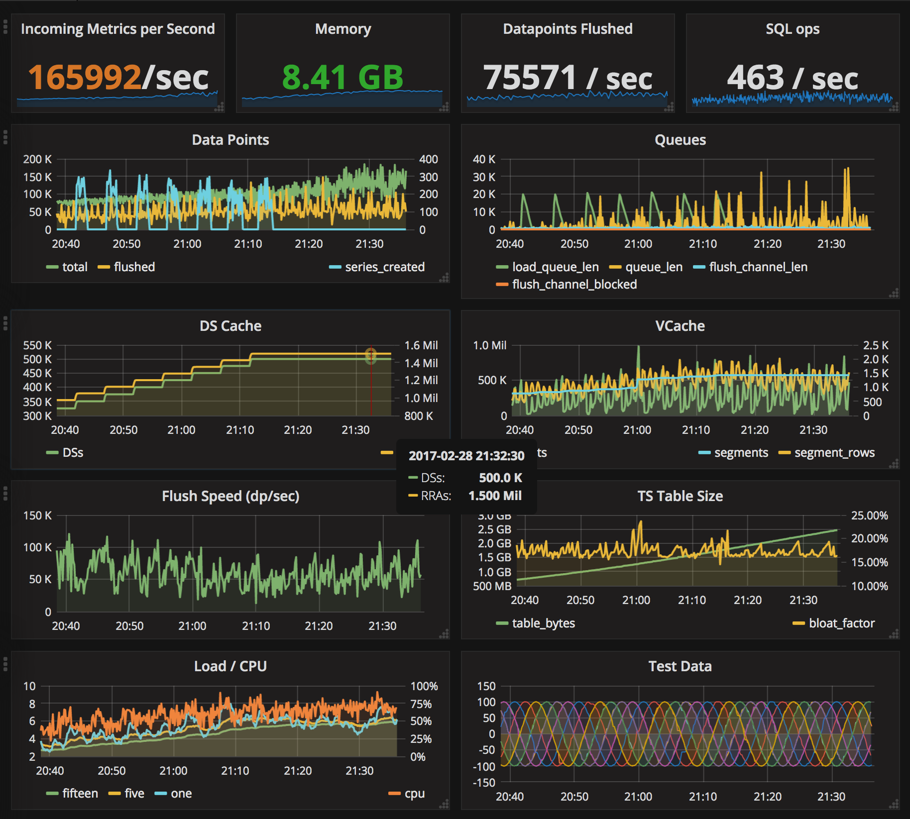
To follow up on the previous post, after a bunch of tweaking, here is Tgres (commit) receiving over 150,000 data points per second across 500,000 time series without any signs of the queue size or any other resource blowing up.

This is both Tgres and Postgres running on the same i2.2xlarge EC2 instance (8 cores, 64GB, SSD).

At this point I think there’s been enough load testing and optimization, and I am going to get back to crossing the t’s and dotting the i’s so that we can release the first version of Tgres.

Note: there is an update to this post.

TL;DR

On a 8 CPU / 16 GB EC2 instance, Tgres can process 150,000 data points per second across 300,000 series (Postgres running on the same machine). With some tweaks we were able to get the number of series to half a million, flushing ~60K data points per second.

Now the long version…

If you were to ask me whether Tgres could outperform Graphite, just a couple of months ago my answer would have been “No”. Tgres uses Postgres to store time series data, while Graphite stores data by writing to files directly, the overhead of the relational database just seemed too great.

Well, I think I’ve managed to prove myself wrong. After re-working Tgres to use the write-optimized layout, I’ve run some tests on AWS yielding unexpectedly promising results.

As a benchmark I targeted the excellent blog post by Jason Dixon describing his AWS Graphite test. My goal was to get to at least half the level of performance described therein. But it appears the combination of Go, Postgres and some clever data structuring has been able to beat it, not without breaking a little sweat, but it has.

My test was conducted on a c4.2xlarge instance, which has 8 cores and 16 GB, using 100GB EBS (which, if I understood it correctly, comes with 300 IOPS, please comment if I’m wrong). The “c4” instances are supposed to be some of the highest speed CPU AWS has to offer, but compare this with the instance used in the Graphite test, an i2.4xlarge (16 CPU/ 122GB), it had half the CPU cores and nearly one tenth of the RAM.

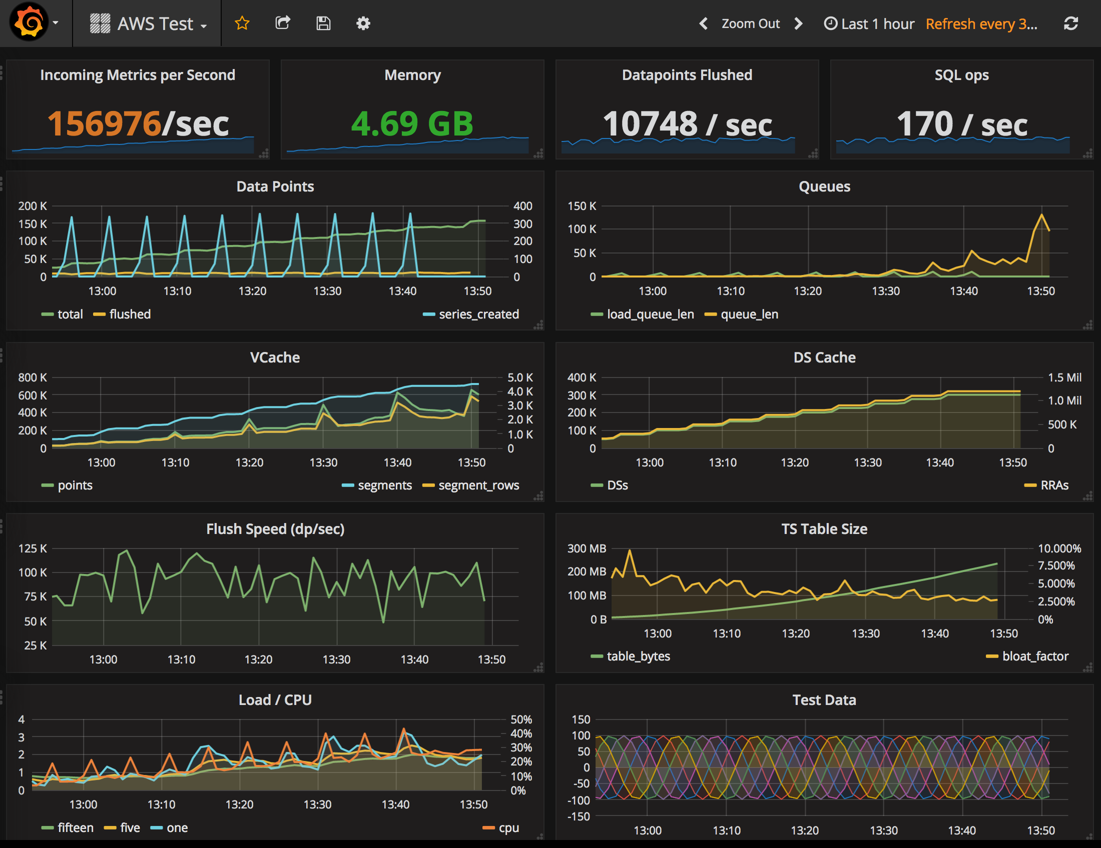
Before I go any further, here is the obligatory screenshot, then my observations and lessons learned in the process, as well as a screenshot depicting even better performance.

The Tgres version running was this one, with the config detailed at the bottom of the post.

Postgres was whatever yum install postgresql95-server brings your way, with the data directory moved to the EBS volume formatted using ext4 (not that I think it matters). The Postgres config was modified to allow a 100ms commit delay and to make autovacuum extra aggressive. I did not increase any memory buffers and left everything else as is. Specifically, these were the changes:

1
2
3
4
5
6
7
8

autovacuum_work_mem = -1
synchronous_commit = off
commit_delay = 100000
autovacuum_max_workers = 10
autovacuum_naptime = 1s
autovacuum_vacuum_threshold = 2000
autovacuum_vacuum_scale_factor = 0.0
autovacuum_vacuum_cost_delay = 0

The data points for the test were generated by a goroutine in the Tgres process itself. In the past I’ve found that blasting a server with this many UDP packets can be tricky and hardware/network intensive. It’s also hard to tell when/if they get dropped and why, etc. Since Go is not known for having problems in its network stack, I was not too worried about it, I just wanted a reliable and configurable source of incoming packets, and in Go world writing a simple goroutine seemed like the right answer.

Somewhat Random Notes and Making Tgres Even Faster

Determining failure

Determining when we are “at capacity” is tricky. I’ve mostly looked at two factors (aside from the obvious - running out of memory/disk, becoming unresponsive, etc): receiver queue size and Postgres table bloat.

Queue size

Tgres uses “elastic channels” (so eloquently described here by Nick Patavalis) for incoming data points and to load series from Postgres. These are channel-like structures that can grow to arbitrary length only limited by the memory available. This is done so as to be able to take maximum advantage of the hardware at hand. If any of those queues starts growing out of control, we are failing. You can see in the picture that at about 140K data points per second the receiver queue started growing, though it did stay steady at this size and never spun out of control (the actual test was left overnight at this rate just to make sure).

PG Table Bloat

Table bloat is a phenomenon affecting Postgres in write-intensive situations because of its adherence to the MVCC. It basically means that pages on disk are being updated faster than the autovacuum process can keep up with them and the table starts growing out of control.

To monitor for table bloat, I used a simple formula which determined the approximate size of the table based on the row count (our data is all floats, which makes it very predictable) and compared it with the actual size. If the actual size exceeded the estimated size, that’s considered bloat. Bloat is reported in the “TS Table Size” chart. A little bloat is fine, and you can see that it stayed in fairly low percent throughout the test.

In the end, though more research is warranted, it may just turn out that contrary to every expectation PostgreSQL was not the limiting factor here. The postmaster processes stayed below 170MB RSS, which is absolutely remarkable, and Grafana refreshes were very quick even at peak loads.

Memory consumption

Tgres has a slight limitation in that creating a series is expensive. It needs to check with Postgres and for reasons I don’t want to bore you with it’s always a SELECT, optionally followed by an “UPSERT”. This takes time, and during the ramp-up period when the number of series is growing fast and lots of them need to be created, the Go runtime ends up consuming a lot of memory. You can see that screenshot image reports 4.69GB. If I were to restart Tgres (which would cause all existing DS names to be pre-cached) its memory footprint stayed at about 1.7GB. More work needs to be done to figure out what accounts for the difference.

Data Point Rate and Number of Series

The rate of data points that need to be saved to disk is a function of the number of series and the resolution of the RRAs. To illustrate, if I have one series at 1 point per second, even if I blast a million data points per second, still only 1 data point per second needs to be saved.

There is an important difference between Graphite and Tgres in that Tgres actually adjusts the final value considering the every data point value using weighted mean, while Graphite just ignores all points but the last. So Tgres does a bit more work, which adds up quickly at 6-figure rates per second.

The Graphite test if I read the chart correctly was able to process ~70K data points per second across 300K series. My test had 300K series and data points were coming in at over 150K/s. But just out of curiosity, I tried to push it to its limit.

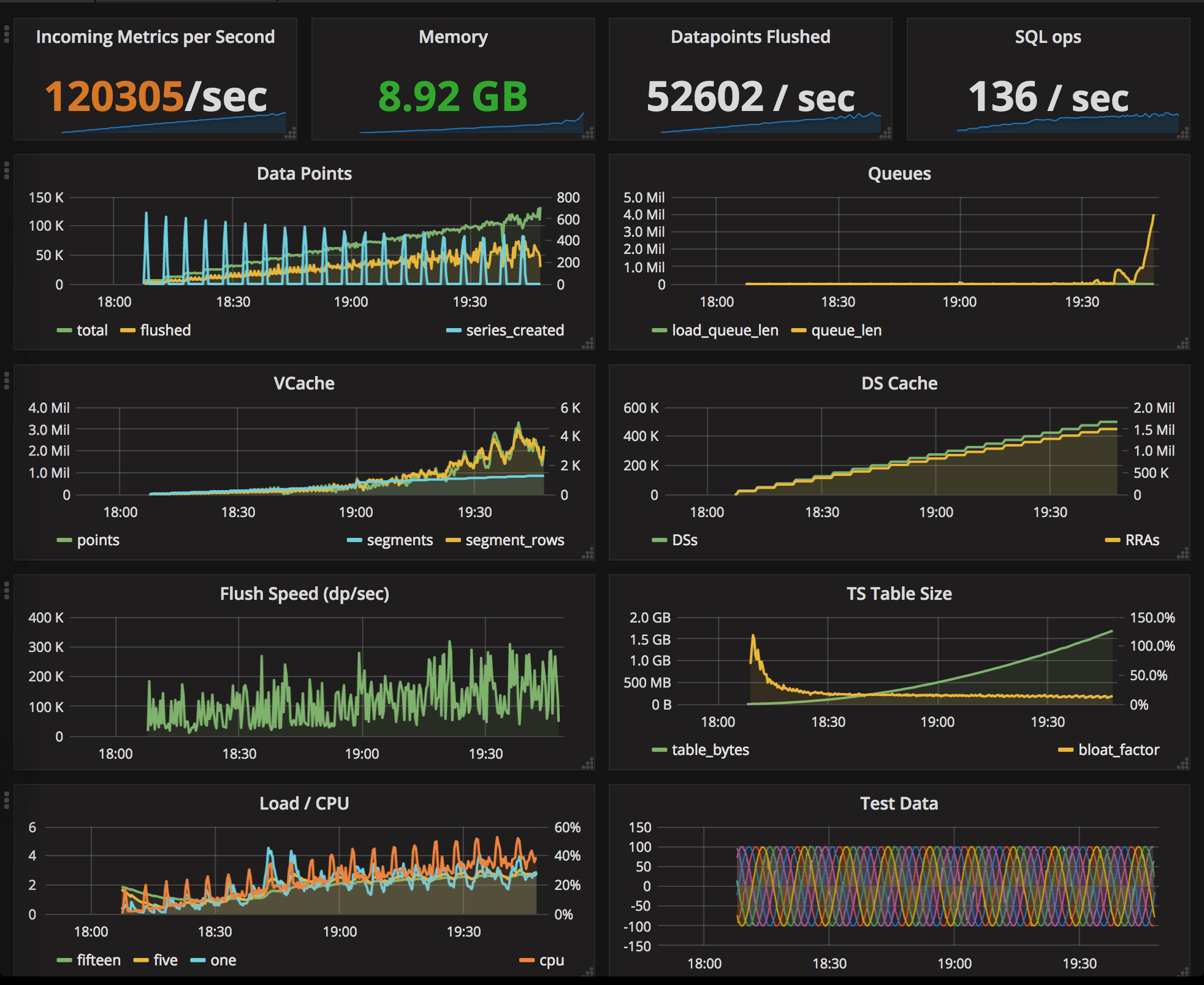
At 400 series, you can see clear signs of deterioration. You can see how vcache isn’t flushed fast enough leaving gaps at the end of series. If we stop the data blast, it does eventually catch up, so long as there is memory for the cache.

If you don’t catch this condition in time, Tgres will die with:

1
2
3
4
5
6

fatal error: runtime: out of memory

runtime stack:
runtime.throw(0xa33e5a, 0x16)
        /home/grisha/.gvm/gos/go1.8/src/runtime/panic.go:596 +0x95
...

Segment Width

There is still one easy performance card we can play here. Segment width is how many data points are stored in one row, it is also the limit on how many points we can transfer in a single SQL operation. Segment width by default is 200, because a width higher than that causes rows to exceed a page and trigger TOAST. TOAST can be good or bad because it means data is stored in a separate table (not so good), but it also means it’s compressed, which may be an I/O win.

So what would happen if we set the segment width to 1000?

The picture changes significantly (see below). I was able to get the number of series to 500K, note the whopping 52,602 data points being written to the database per second! You can see we’re pushing it to the limit because the receiver queue is beginning to grow. I really wanted to get the rate up to 150K/sec, but it just didn’t want to go there.

And what would happen if we set the segment width to 4096?

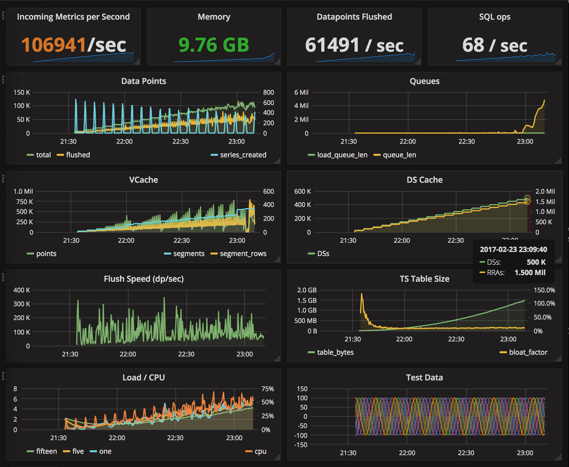
Interestingly, the memory footprint is a tad larger while the vcache is leaner, the number of data points flushed per second is about same, though in fewer SQL statements, and the overall picture is about the same and the incoming queue still skyrockets at just about 100K/sec over 500K series.

Conclusion

There is plenty of places in Tgres code that could still be optimized.

One issue that would be worth looking into is exposing Tgres to the firehose on an empty database. The current code runs out of memory in under a minute when suddenly exposed to 300K new series at 150K/s. Probably the simplest solution to this would be to somehow detect that we’ve unable to keep up and start dropping data points. Eventually, when all the series are created and cached, performance should even out after the initial spike and all should be well.

In any event, it’s nice to be able to do something like this and know that it is performant as well:

1
2
3
4
5
6
7
8
9
10
11
12
13
14

tgres=> select t, r from ds
 join tv  on tv.ds_id = ds.id
where ident @> '{"name":"tgres.0_0_0_0.runtime.load.five"}'
  and tv.step_ms = 10000
order by t desc
limit 5;
           t            |       r
------------------------+----------------
 2017-02-23 22:31:50+00 | 1.256833462648
 2017-02-23 22:26:30+00 | 1.305209492142
 2017-02-23 22:24:10+00 | 1.554056287975
 2017-02-23 22:24:00+00 | 1.453365774931
 2017-02-23 22:23:50+00 | 1.380504724386
(5 rows)

Reference

For completness sake, the instance was created using Terraform config approximately like this:

1
2
3
4
5
6
7
8
9
10
11
12
13
14
15
16
17
18
19
20
21
22
23
24
25
26
27
28
29

variable "aws_region" { default = "us-east-1" }
variable "aws_zone" { default = "us-east-1a" }
variable "key_name" { default = "REDACTED"

provider "aws" {
  region = "${var.aws_region}"
}

resource "aws_ebs_volume" "ebs_volume" {
  availability_zone = "${var.aws_zone}"
  size = 100
}

resource "aws_volume_attachment" "ebs_att" {
  device_name = "/dev/sdh"
  volume_id = "${aws_ebs_volume.ebs_volume.id}"
  instance_id = "${aws_instance.tgres-test-tmp.id}"
}

resource "aws_instance" "tgres-test-tmp" {
  ami = "ami-0b33d91d"
  instance_type = "c4.2xlarge"
  subnet_id = "REDACTED"
  vpc_security_group_ids = [
    "REDACTED"
  ]
  associate_public_ip_address = true
  key_name = "${var.key_name}"
}

And then the following commands were used to prime everyting:

1
2
3
4
5
6
7
8
9
10
11
12
13
14
15
16
17
18
19
20
21
22
23
24
25
26
27
28
29
30
31
32
33
34
35
36
37
38
39

sudo mke2fs /dev/sdh
sudo mkdir /ebs
sudo mount /dev/sdh /ebs

sudo yum install -y postgresql95-server
sudo service postgresql95 initdb
sudo mkdir /ebs/pg
sudo mv /var/lib/pgsql95/data /ebs/pg/data
sudo ln -s /ebs/pg/data /var/lib/pgsql95/data

sudo vi /var/lib/pgsql95/data/postgresql.conf
# BEGIN postgres config - paste this somewhere in the file
autovacuum_work_mem = -1
synchronous_commit = off
commit_delay = 100000
autovacuum_max_workers = 10
autovacuum_naptime = 1s
autovacuum_vacuum_threshold = 2000
autovacuum_vacuum_scale_factor = 0.0
autovacuum_vacuum_cost_delay = 0
# END postgres config

sudo service postgresql95 restart

# create PG database

sudo su - postgres
createuser -s ec2-user   # note -s is superuser - not necessary for tgres but just in case
createdb tgres
exit

# Tgres (requires Go - I used 1.8)
# (or you can just scp it from some machine where you already have go environment)
mkdir golang
export GOPATH=~/golang/
go get github.com/tgres/tgres
cd /home/ec2-user/golang/src/github.com/tgres/tgres
go build
cp etc/tgres.conf.sample etc/tgres.conf

The tgres.conf file looked like this:

1
2
3
4
5
6
7
8
9
10
11
12
13
14
15
16
17
18
19
20
21
22
23
24
25
26
27

min-step                = "10s"

pid-file =                 "tgres.pid"
log-file =                 "log/tgres.log"
log-cycle-interval =       "24h"

max-flushes-per-second      = 1000000 # NB - Deprecated setting
workers                     = 4       # NB - Deprecated setting

http-listen-spec            = "0.0.0.0:8888"
graphite-line-listen-spec   = "0.0.0.0:2003"
graphite-text-listen-spec   = "0.0.0.0:2003"
graphite-udp-listen-spec    = "0.0.0.0:2003"
graphite-pickle-listen-spec = "0.0.0.0:2004"

statsd-text-listen-spec     = "0.0.0.0:8125"
statsd-udp-listen-spec      = "0.0.0.0:8125"
stat-flush-interval         = "10s"
stats-name-prefix           = "stats"

db-connect-string = "host=/tmp dbname=tgres sslmode=disable"

[[ds]]
regexp = ".*"
step = "10s"
#heartbeat = "2h"
rras = ["10s:6h", "1m:7d", "1h:1y"]

Tgres was running with the following. The TGRES_BLASTER starts the blaster goroutine.

1

TGRES_BIND=0.0.0.0 TGRES_BLASTER=1 ./tgres

Once you have Tgres with the blaster running, you can control it via HTTP, e.g. the following would set it to 50K/s data points across 100K series. Setting rate to 0 pauses it.

1

curl -v "http://127.0.0.1:8888/blaster/set?rate=50000&n=100000"

Continuing on the previous write up on how time series data can be stored in Postgres efficiently, here is another approach, this time providing for extreme write performance.

The “horizontal” data structure in the last article requires an SQL statement for every data point update. If you cache data points long enough, you might be able to collect a bunch for a series and write them out at once for a slight performance advantage. But there is no way to update multiple series with a single statement, it’s always at least one update per series. With a large number of series, this can become a performance bottleneck. Can we do better?

One observation we can make about incoming time series data is that commonly the data points are roughly from the same time period, the current time, give or take. If we’re storing data at regularly-spaced intervals, then it is extremely likely that many if not all of the most current data points from various time series are going to belong to the exact same time slot. Considering this observation, what if we organized data points in rows of arrays, only now we would have a row per timestamp while the position within the array would determine the series?

Lets create the tables:

1
2
3
4
5
6
7
8
9
10
11
12
13
14
15
16
17

CREATE TABLE rra_bundle (
  id SERIAL NOT NULL PRIMARY KEY,
  step_ms INT NOT NULL,
  steps_per_row INT NOT NULL,
  size INT NOT NULL,
  latest TIMESTAMPTZ DEFAULT NULL);

CREATE TABLE rra (
  id SERIAL NOT NULL PRIMARY KEY,
  ds_id INT NOT NULL,
  rra_bundle_id INT NOT NULL,
  pos INT NOT NULL);

CREATE TABLE ts (
  rra_bundle_id INT NOT NULL,
  i INT NOT NULL,
  dp DOUBLE PRECISION[] NOT NULL DEFAULT '{}');

Notice how the step and size now become properties of the bundle rather than the rra which now refers to a bundle. In the ts table, i is the index in the round-robin archive (which in the previous “horizontal” layout would be the array index).

The data we used before was a bunch of temperatures, lets add two more series, one where temperature is 1 degree higher, and one where it’s 1 degree lower. (Not that it really matters).

1
2
3
4
5
6
7
8
9
10
11
12
13
14
15
16
17
18
19
20
21
22
23
24
25
26
27
28
29
30
31
32
33
34

INSERT INTO rra_bundle VALUES (1, 60000, 1440, 28, '2008-04-02 00:00:00-00');

INSERT INTO rra VALUES (1, 1, 1, 1);
INSERT INTO rra VALUES (2, 2, 1, 2);
INSERT INTO rra VALUES (3, 3, 1, 3);

INSERT INTO ts VALUES (1, 0, '{64,65,63}');
INSERT INTO ts VALUES (1, 1, '{67,68,66}');
INSERT INTO ts VALUES (1, 2, '{70,71,69}');
INSERT INTO ts VALUES (1, 3, '{71,72,70}');
INSERT INTO ts VALUES (1, 4, '{72,73,71}');
INSERT INTO ts VALUES (1, 5, '{69,70,68}');
INSERT INTO ts VALUES (1, 6, '{67,68,66}');
INSERT INTO ts VALUES (1, 7, '{65,66,64}');
INSERT INTO ts VALUES (1, 8, '{60,61,59}');
INSERT INTO ts VALUES (1, 9, '{58,59,57}');
INSERT INTO ts VALUES (1, 10, '{59,60,58}');
INSERT INTO ts VALUES (1, 11, '{62,63,61}');
INSERT INTO ts VALUES (1, 12, '{68,69,67}');
INSERT INTO ts VALUES (1, 13, '{70,71,69}');
INSERT INTO ts VALUES (1, 14, '{71,72,70}');
INSERT INTO ts VALUES (1, 15, '{72,73,71}');
INSERT INTO ts VALUES (1, 16, '{77,78,76}');
INSERT INTO ts VALUES (1, 17, '{70,71,69}');
INSERT INTO ts VALUES (1, 18, '{71,72,70}');
INSERT INTO ts VALUES (1, 19, '{73,74,72}');
INSERT INTO ts VALUES (1, 20, '{75,76,74}');
INSERT INTO ts VALUES (1, 21, '{79,80,78}');
INSERT INTO ts VALUES (1, 22, '{82,83,81}');
INSERT INTO ts VALUES (1, 23, '{90,91,89}');
INSERT INTO ts VALUES (1, 24, '{69,70,68}');
INSERT INTO ts VALUES (1, 25, '{75,76,74}');
INSERT INTO ts VALUES (1, 26, '{80,81,79}');
INSERT INTO ts VALUES (1, 27, '{81,82,80}');

Notice that every INSERT adds data for all three of our series in a single database operation!

Finally, let us create the view. (How it works is described in detail in the previous article)

1
2
3
4
5
6
7
8
9

CREATE VIEW tv AS
  SELECT rra.id as rra_id,
     rra_bundle.latest - INTERVAL '1 MILLISECOND' * rra_bundle.step_ms * rra_bundle.steps_per_row *
       MOD(rra_bundle.size + MOD(EXTRACT(EPOCH FROM rra_bundle.latest)::BIGINT*1000/(rra_bundle.step_ms * rra_bundle.steps_per_row),
       rra_bundle.size) - i, rra_bundle.size) AS t,
     dp[pos] AS r
  FROM rra AS rra
  JOIN rra_bundle AS rra_bundle ON rra_bundle.id = rra.rra_bundle_id
  JOIN ts AS ts ON ts.rra_bundle_id = rra_bundle.id;

And now let’s verify that it works:

1
2
3
4
5
6
7
8

=> select * from tv where rra_id = 1 order by t;
 rra_id |           t            | r
 --------+------------------------+----
       1 | 2008-03-06 00:00:00-00 | 64
       1 | 2008-03-07 00:00:00-00 | 67
       1 | 2008-03-08 00:00:00-00 | 70
 ...

This approach makes writes blazingly fast though it does have its drawbacks. For example there is no way to read a single series - even though the view selects a single array element, under the hood Postgres reads the whole row. Given that time series is more write intensive and rarely read, this may not be a bad compromise.

Continuing on the the previous post on simple use of Tgres components, let’s try to count something that goes by really fast.

This time let’s start out with creating a memory-based SerDe. This means that all our data is in memory and there is no database backing our series.

1
2
3
4
5
6
7
8
9
10
11
12
13
14
15
16
17
18
19
20
21
22
23
24
25
26
27
28
29
30
31
32
33

package main

import (
    "fmt"
    "net/http"
    "time"

    "github.com/tgres/tgres/dsl"
    h "github.com/tgres/tgres/http"
    "github.com/tgres/tgres/receiver"
    "github.com/tgres/tgres/rrd"
    "github.com/tgres/tgres/serde"
)

func main() {

    step := 1 * time.Second // 1 second resolution
    span := 600 * step      // spanning 10 minutes

    // In-memory SerDe
    ms := serde.NewMemSerDe()

    // Create a receiver of our data points backed by the above
    // memory SerDe
    rcvr := receiver.New(ms, &receiver.SimpleDSFinder{&rrd.DSSpec{
        Step: step,
        RRAs: []rrd.RRASpec{
            rrd.RRASpec{Function: rrd.WMEAN,
                Step: step,
                Span: span,
            },
        }}})
    rcvr.Start()

Now let’s create a goroutine which creates data points as fast as it can, the difference from the previous blog post is that we are using QueueGauge(), which is a paced metric, meaning that it flushes to the time series only periodically (once per second by default) so as to not overwhelm the I/O and or network (even though in this case it doesn’t really matter since we’re using a memory-based SerDe anyway).

1
2
3
4
5
6
7
8
9
10

    start := time.Now()
    end := start.Add(span)

    go func() {
        n := 0
        for t := time.Now(); t.Before(end); t = time.Now() {
            rcvr.QueueGauge(serde.Ident{"name":"foo.bar"}, float64(n)/(t.Sub(start)).Seconds())
            n++
        }
    }()

And finally, as before, we need to hook up a couple of http handlers:

1
2
3
4
5
6
7
8
9
10

    db := dsl.NewNamedDSFetcher(ms.Fetcher())

    http.HandleFunc("/metrics/find", h.GraphiteMetricsFindHandler(db))
    http.HandleFunc("/render", h.GraphiteRenderHandler(db))

    listenSpec := ":8088"
    fmt.Printf("Waiting for requests on %s\n", listenSpec)
    http.ListenAndServe(listenSpec, nil)

} // end of main()

Now if we run the above code with something like go run simpletgres.go, we’ll notice that unlike with the previous example, the web server starts right away, and the data points are being written while the server is running. If we aim Grafana at it, we should be able to see the chart update in real time.

After a couple of minutes, mine looks like this:

So my macbook can crank these out at about 2.5 million per second.

In my experience instrumenting my apps with simple counters like this and having them available directly from the app without having to send them to a separate statsd server somewhere has been extremely useful in helping understand performance and other issues.

If you’re reading this, chances are you may have searched for definition of “Time Series”. And, like me, you were probably disappointed by what you’ve found.

The most popular “definition” I come across amongst our fellow programmer folk is that it’s “data points with timestamps”. Or something like that. And you can make charts from it. And that’s about it, alas.

The word time suggests that is has something to do with time. At first it seems reasonable, I bite. The word series is a little more peculiar. A mathematician would argue that a series is a sum of a sequence. Most people though think “series” and “sequence” are the same thing, and that’s fine. But it’s a clue that time series is not a scientific term, because it would have been called time sequence most likely.

Lets get back to the time aspect of it. Why do data points need timestamps? Or do they? Isn’t it the time interval between points that is most essential, rather than the absolute time? And if the data points are spaced equally (which conforms to the most common definiton of time series), then what purpose would any time-related information attached to a data point serve?

To understand this better, picture a time chart. Of anything - temperature, price of bitcoin over a week, whatever. Now think - does the absolute time of every point provide any useful information to you? Does the essential meaning of the chart change depending on whether it shows the price of bitcoin in the year 2016 or 2098 or 10923?

Doesn’t it seem like “time” in “time series” is a bit of a red herring?

Here is another example. Let’s say I decide to travel from San-Francisco to New York taking measurements of elevation above the sea level at every mile. I then plot that sequence on a chart where x-axis is distance traveled and y-axis is elevation. You would agree that this chart is not a “time series” by any stretch, right? But then if I renamed x-axis to “time traveled” (let’s assume I moved at constant speed), the chart wouldn’t change at all, but now it’s okay to call it “time series”?

So it’s no surprise that there is no formal definition of “time series”. In the end a “time series” is just a sequence. There are no timestamps required and there is nothing at all special regarding a dimension being time as opposed to any other unit, which is why there is no mathematical definition of “time series”. Time series is a colloquial term etymological origins of which are not known to me, but it’s not a thing from a scientific perspective, I’m afraid.

Next time you hear “time series” just substitute it with “sequence” and see how much sense that makes. For example a “time series database” is a “sequence database”, i.e. database optimized for sequences. Aren’t all relational databases optimized for sequences?

Something to think about over the holidays…

Edit: Someone brought up the subject of unevenly-spaced time series. All series are evenly spaced given proper resolution. An unevenly-spaced time series with timestamps accurate to 1 millisecond is a sparse evenly-spaced series with a 1 millisecond resolution.

Did you know you can use Tgres components in your code without PostgreSQL, and in just a dozen lines of code instrument your program with a time series. This example shows a complete server emulating Graphite API which you can use with Grafana (or any other tool).

In this example we will be using three Tgres packages like so (in addition to a few standard ones, I’m skipping them here for brevity - complete source code gist):

1
2
3
4
5

import (
    "github.com/tgres/tgres/dsl"
    h "github.com/tgres/tgres/http"
    "github.com/tgres/tgres/rrd"
)

First we need a Data Source. This will create a Data Source containing one Round Robin Archive with a 10 second resolution spanning 1000 seconds.

1
2
3
4
5
6
7
8
9

step := 10 * time.Second
span := 100 * step

ds := rrd.NewDataSource(rrd.DSSpec{
    Step: 1 * time.Second,
    RRAs: []rrd.RRASpec{
        rrd.RRASpec{Step: step, Span: span},
    },
})

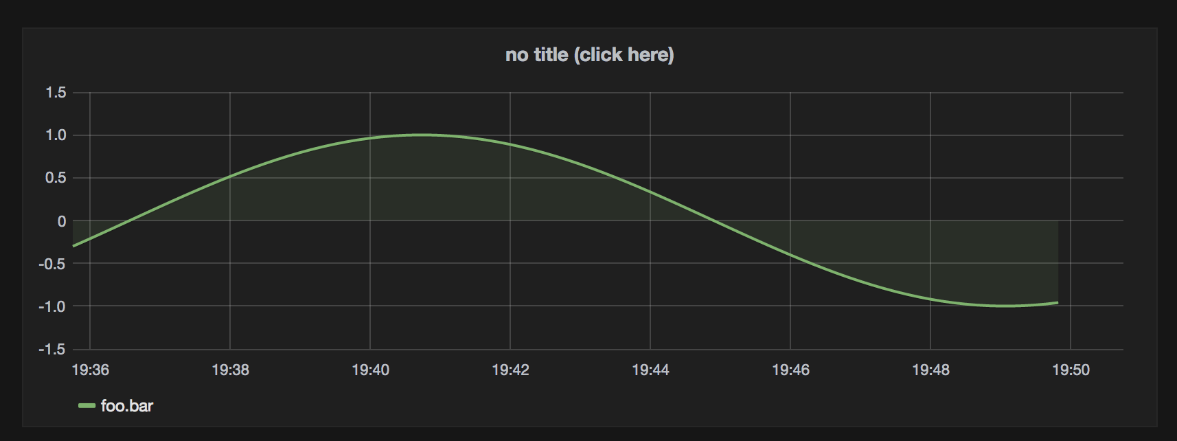
Let’s shove a bunch of data points into it. To make it look extra nice, we can make these points look like a sinusoid with this little function:

1
2
3
4

func sinTime(t time.Time, span time.Duration) float64 {
    x := 2 * math.Pi / span.Seconds() * float64(t.Unix()%(span.Nanoseconds()/1e9))
    return math.Sin(x)
}

And now for the actual population of the series:

1
2
3
4
5
6

start := time.Now().Add(-span)

for i := 0; i < int(span/step); i++ {
    t := start.Add(time.Duration(i) * step)
    ds.ProcessDataPoint(sinTime(t, span), t)
}

We will also need to create a NamedDSFetcher, the structure which knows how to search dot-separated series names a la Graphite.

1

db := dsl.NewNamedDSFetcherMap(map[string]rrd.DataSourcer{"foo.bar": ds})

Finally, we need to create two http handlers which will mimic a Graphite server and start listening for requests:

1
2
3
4
5
6

http.HandleFunc("/metrics/find", h.GraphiteMetricsFindHandler(db))
http.HandleFunc("/render", h.GraphiteRenderHandler(db))

listenSpec := ":8088"
fmt.Printf("Waiting for requests on %s\n", listenSpec)
http.ListenAndServe(listenSpec, nil)

Now if you point Grafana at it, it will happily think it’s Graphite and should show you a chart like this:

Note that you can use all kinds of Graphite functions at this point - it all “just works”.

Enjoy!