If you haven’t read Part I and Part II you probably should, or the following will be hard to make sense of.

In Part I we’ve learned how to forceast one point, in Part II we’ve learned how to forecast two points. In this part we’ll learn how to forecast many points.

More Terminology

Season

If a series appears to be repetitive at regular intervals, such an interval is referred to as a season, and the series is said to be seasonal. Seasonality is required for the Holt-Winters method to work, non-seasonal series (e.g. stock prices) cannot be forecasted using this method (would be nice though if they could be).

Season Length

Season length is the number of data points after which a new season begins. We will use $L$ to denote season length.

Seasonal Component

The seasonal component is an additional deviation from level + trend that repeats itself at the same offset into the season. There is a seasonal component for every point in a season, i.e. if your season length is 12, there are 12 seasonal components. We will use $s$ to denote the seasonal component.

Triple Exponential Smoothing a.k.a Holt-Winters Method

The idea behind triple exponential smoothing is to apply exponential smoothing to the seasonal components in addition to level and trend. The smoothing is applied across seasons, e.g. the seasonal component of the 3rd point into the season would be exponentially smoothed with the the one from the 3rd point of last season, 3rd point two seasons ago, etc. In math notation we now have four equations (see footnote):

• What’s new:
  • We now have a third greek letter, $\gamma$ (gamma) which is the smoothing factor for the seasonal component.
  • The expected value index is $x+m$ where $m$ can be any integer meaning we can forecast any number of points into the future (woo-hoo!)
  • The forecast equation now consists of level, trend and the seasonal component.

The index of the seasonal component of the forecast $s_{x-L+1+(m-1)modL}$ may appear a little mind boggling, but it’s just the offset into the list of seasonal components from the last set from observed data. (I.e. if we are forecasting the 3rd point into the season 45 seasons into the future, we cannot use seasonal components from the 44th season in the future since that season is also forecasted, we must use the last set of seasonal components from observed points, or from “the past” if you will.) It looks much simpler in Python as you’ll see shortly.

Initial Values

Before we can discuss initial values, let me introduce to you a new tiny series (okay, not as tiny):

1
2
3
4

series = [30,21,29,31,40,48,53,47,37,39,31,29,17,9,20,24,27,35,41,38,
          27,31,27,26,21,13,21,18,33,35,40,36,22,24,21,20,17,14,17,19,
          26,29,40,31,20,24,18,26,17,9,17,21,28,32,46,33,23,28,22,27,
          18,8,17,21,31,34,44,38,31,30,26,32]

This is what it looks like:

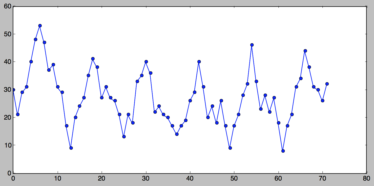
You can see that this series is seasonal, there are clearly visible 6 seasons. Although perhaps not easily apparent from the picture, the season length for this series is 12, i.e. it “repeats” every 12 points. In order to apply triple exponential smoothing we need to know what the season length is. (There do exist methods for detecting seasonality in series, but this is way beyond the scope of this text).

Initial Trend

For double exponential smoothing we simply used the first two points for the initial trend. With seasonal data we can do better than that, since we can observe many seasons and can extrapolate a better starting trend. The most common practice is to compute the average of trend averages across seasons.

Good news - this looks simpler in Python than in math notation:

1
2
3
4
5
6
7
8

def initial_trend(series, slen):
    sum = 0.0
    for i in range(slen):
        sum += float(series[i+slen] - series[i]) / slen
    return sum / slen

# >>> initial_trend(series, 12)
# -0.7847222222222222

Initial Seasonal Components

The situation is even more complicated when it comes to initial values for the seasonal components. Briefly, we need to compute the average level for every observed season we have, divide every observed value by the average for the season it’s in and finally average each of these numbers across our observed seasons. If you want more detail, here is one thorough description of this process.

I will forgo the math notation for initial seasonal components, but here it is in Python. The result is a season-length array of seasonal components.

1
2
3
4
5
6
7
8
9
10
11
12
13
14
15
16
17

def initial_seasonal_components(series, slen):
    seasonals = {}
    season_averages = []
    n_seasons = int(len(series)/slen)
    # compute season averages
    for j in range(n_seasons):
        season_averages.append(sum(series[slen*j:slen*j+slen])/float(slen))
    # compute initial values
    for i in range(slen):
        sum_of_vals_over_avg = 0.0
        for j in range(n_seasons):
            sum_of_vals_over_avg += series[slen*j+i]-season_averages[j]
        seasonals[i] = sum_of_vals_over_avg/n_seasons
    return seasonals

# >>> initial_seasonal_components(series, 12)
# {0: -7.4305555555555545, 1: -15.097222222222221, 2: -7.263888888888888, 3: -5.097222222222222, 4: 3.402777777777778, 5: 8.069444444444445, 6: 16.569444444444446, 7: 9.736111111111112, 8: -0.7638888888888887, 9: 1.902777777777778, 10: -3.263888888888889, 11: -0.7638888888888887}

The Algorithm

And finally, here is the additive Holt-Winters method in Python. The arguments to the function are the series of observed values, the season length, alpha, beta, gamma and the number of points we want forecasted.:

1
2
3
4
5
6
7
8
9
10
11
12
13
14
15
16
17
18
19
20
21
22
23

def triple_exponential_smoothing(series, slen, alpha, beta, gamma, n_preds):
    result = []
    seasonals = initial_seasonal_components(series, slen)
    for i in range(len(series)+n_preds):
        if i == 0: # initial values
            smooth = series[0]
            trend = initial_trend(series, slen)
            result.append(series[0])
            continue
        if i >= len(series): # we are forecasting
            m = i - len(series) + 1
            result.append((smooth + m*trend) + seasonals[i%slen])
        else:
            val = series[i]
            last_smooth, smooth = smooth, alpha*(val-seasonals[i%slen]) + (1-alpha)*(smooth+trend)
            trend = beta * (smooth-last_smooth) + (1-beta)*trend
            seasonals[i%slen] = gamma*(val-smooth) + (1-gamma)*seasonals[i%slen]
            result.append(smooth+trend+seasonals[i%slen])
    return result

# # forecast 24 points (i.e. two seasons)
# >>> triple_exponential_smoothing(series, 12, 0.716, 0.029, 0.993, 24)
# [30, 20.34449316666667, 28.410051892109554, 30.438122252647577, 39.466817731253066, ...

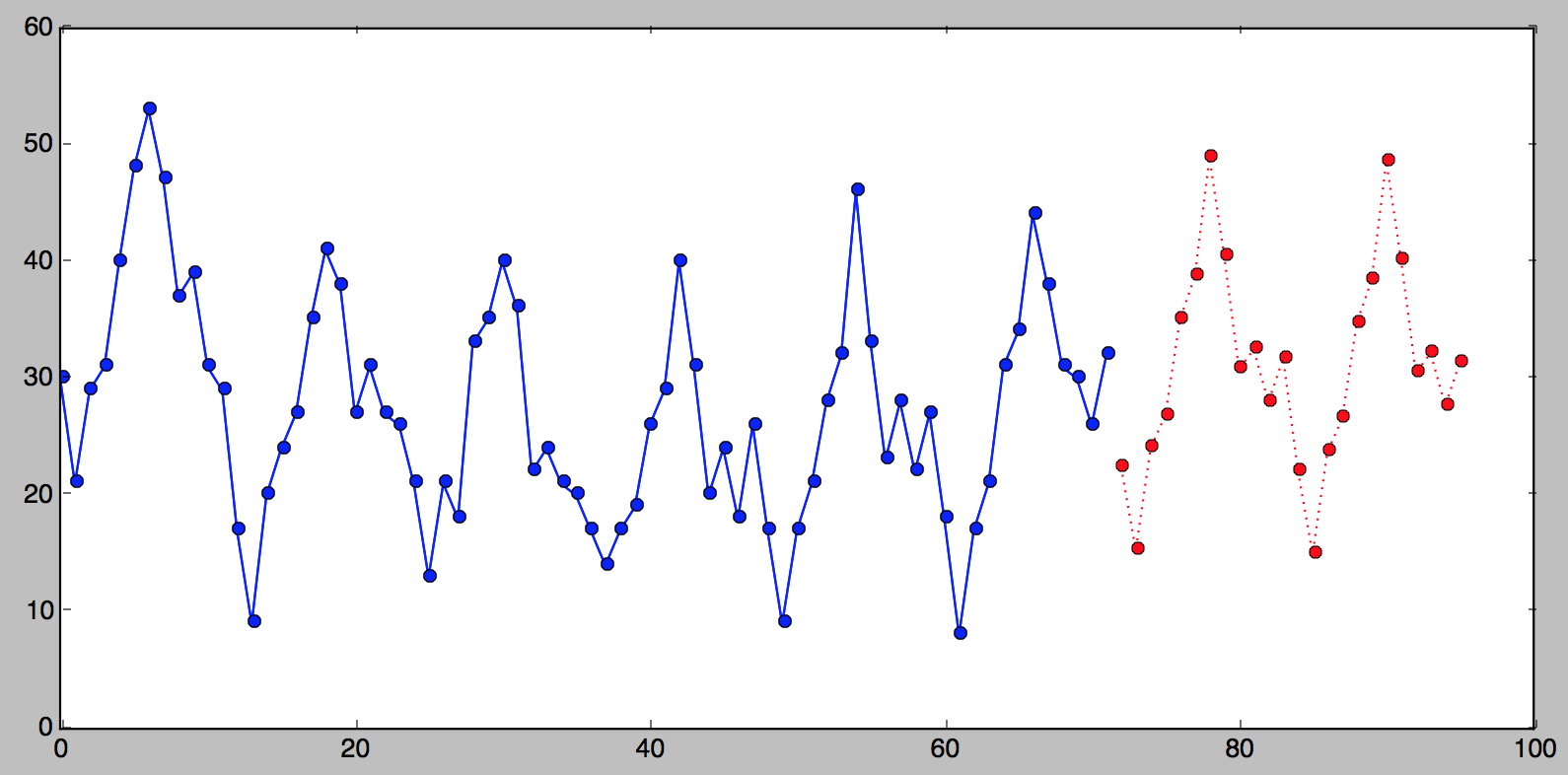
And here is what this looks like if we were to plot the original series, followed by the last 24 points from the result of the triple_exponential_smoothing() call:

A Note on α, β and γ

You may be wondering how I came up with 0.716, 0.029 and 0.993 for $\alpha$, $\beta$ and $\gamma$, respectively. To make long story short, it was done by way of trial and error: simply running the algorithm over and over again and selecting the values that give you the smallest SSE. As I mentioned before, this process is known as fitting.

To compute the smothing factors to three decimal points we may have to run through 1,000,000,000 iterations, but luckily there are more efficient methods at zooming in on best values. Unfortunately this would take a whole other very long post to describe this process. One good algorithm for this is Nelder-Mead, which is what tgres uses.

Conclusion

Well - here you have it, Holt-Winters method explained the way I wish it would have been explained to me when I needed it. If you think I missed something, found an error or a suggestion, please do not hesitate to comment!

Footnote

The triple exponential smoothing additive method formula is as it is described in “Forecasting Method and Applications, Third Edition” by Makridakis, Wheelwright and Hyndman (1998). Wikipedia has a different formula for the seasonal component (I don’t know which is better):